1D Slab Benchmark: Neutron Transport Coupled With Thermal Conduction and Material Expansion

This verification problem demonstrates the ability to couple neutron transport with thermal conduction and material expansion. The analytic benchmark slab problem (Griesheimer and Kooreman, 2022) describes a slab where S $var element = document.getElementById("moose-equation-32ea0c2e-0780-4c0d-8a05-6f036bcc73c6");katex.render("_2", element, {displayMode:false,throwOnError:false});$ neutron transport is coupled with thermal conduction, convective boundary conditions, Doppler-broadened cross sections, and nonlinear thermal expansion effects along the heated slab. The verification provides the analytic solutions for steady-state temperature, neutron flux, heating, multiplication factor, and the heated slab length.

While the restriction to S $var element = document.getElementById("moose-equation-937fbcd7-7e5d-4830-b81e-a43434dc44b1");katex.render("_2", element, {displayMode:false,throwOnError:false});$ neutron transport would be considered overly simplistic for most radiation transport simulations, the objective here is to verify thermomechanical-OpenMC coupling using analytic solutions for three coupled solution fields (displacements, temperature, and flux). Simplifications of each individual physics included in this model are not imposed by inherent limitations of the moving-mesh capabilities and only aim to allow the study on the interactions between multiphysics with an analytic solution.

This work was published in Eltawila et al. (2026), where more details can be found.

Problem description

A 1D slab (Griesheimer and Kooreman, 2022) with initial length $var element = document.getElementById("moose-equation-17a24ffd-d10e-4e68-949a-f7b86a9505b3");katex.render("L_0", element, {displayMode:false,throwOnError:false});$ and density $var element = document.getElementById("moose-equation-60d0915f-57d2-4487-b4bb-5b1038d343d8");katex.render("\\rho_0", element, {displayMode:false,throwOnError:false});$ has neutrons traveling with directions $var element = document.getElementById("moose-equation-5ea25e0e-c82b-41ba-a9f7-180d270de526");katex.render("\\mu = \\pm 1", element, {displayMode:false,throwOnError:false});$ and with zero incoming neutron flux boundary conditions on both sides. The slab is mechanically constrained and perfectly insulated in the transverse dimensions (i.e., $var element = document.getElementById("moose-equation-14970dfd-cdf8-445b-9f20-6049867669cb");katex.render("y", element, {displayMode:false,throwOnError:false});$ and $var element = document.getElementById("moose-equation-63725404-ee34-4672-ac7e-03126fdaa423");katex.render("z", element, {displayMode:false,throwOnError:false});$ axes) but free to expand via frictionless sliding along the $var element = document.getElementById("moose-equation-d2f407e2-9276-490b-853c-268cef745dd5");katex.render("x", element, {displayMode:false,throwOnError:false});$ axis as the temperature of the slab changes. Both ends of the slab are exposed to a convective heat sink at a fixed temperature $var element = document.getElementById("moose-equation-520b21cb-28b2-44a2-8816-c969fa3a870c");katex.render("T_0", element, {displayMode:false,throwOnError:false});$ .

The neutron heating in the slab drives the temperature distribution and causes thermal expansion. This slab elongation feeds back into neutronics and heat conduction by influencing the domain length and material density. A schematic of the problem domain and boundary conditions is shown in Figure 1.

Figure 1: Schematic of the three coupled physics.

The benchmark uses a one-group assumption for neutron cross sections. The neutron flux distribution in the slab is governed by quasi-static transport in 1D. The resulting transport equation is

$(1)var element = document.getElementById("moose-equation-7f406375-d6b6-4a02-805a-53ea0dfce280");katex.render(" \\frac{d}{dx}\\left[\\frac{1}{\\Sigma_t(x)}\\frac{d\\phi(x)}{dx} \\right] + (\\lambda -1 ) \\Sigma_t(x)\\phi(x) = 0,", element, {displayMode:true,throwOnError:false});$

where we consider the vacuum flux boundary conditions

$(2)var element = document.getElementById("moose-equation-34233f91-801c-4c2e-8eeb-65b5760f7944");katex.render(" \\pm \\frac{d\\phi}{dx}\\biggr\\rvert_{\\pm L/2} + \\Sigma_t\\left(\\pm \\frac{L}{2}\\right)\\phi\\left(\\pm \\frac{L}{2}\\right) = 0,", element, {displayMode:true,throwOnError:false});$

where $var element = document.getElementById("moose-equation-9b4e6ddd-d21c-4d42-9745-56ede60fa0d9");katex.render("\\phi", element, {displayMode:false,throwOnError:false});$ is the neutron flux, $var element = document.getElementById("moose-equation-fa42202b-2498-4013-aa5e-09b52426e5c1");katex.render("\\Sigma_t", element, {displayMode:false,throwOnError:false});$ is the macroscopic total cross section, and $var element = document.getElementById("moose-equation-e422b59e-9f9d-4292-a452-d669d5fa6cb8");katex.render("\\lambda", element, {displayMode:false,throwOnError:false});$ is the combined in-scattering and (quasi-static) fission source term. $var element = document.getElementById("moose-equation-8b2074f0-13b6-4938-b6fe-3b9c6b800264");katex.render("\\lambda", element, {displayMode:false,throwOnError:false});$ is defined as

$(3)var element = document.getElementById("moose-equation-0c9bf8f2-d973-4aac-9be2-7b834638f876");katex.render(" \\lambda \\equiv \\frac{1}{k_\\text{eff}}\\frac{\\nu\\Sigma_f}{\\Sigma_t}+\\frac{\\Sigma_s}{\\Sigma_t},", element, {displayMode:true,throwOnError:false});$

where $var element = document.getElementById("moose-equation-90f337a5-ac71-4739-8ed2-1c70b5ff4985");katex.render("\\nu", element, {displayMode:false,throwOnError:false});$ is the average number of neutrons released per fission, $var element = document.getElementById("moose-equation-d985512b-8bd1-4568-b2ee-b53e2dbc837a");katex.render("k_\\text{eff}", element, {displayMode:false,throwOnError:false});$ is the multiplication factor, and $var element = document.getElementById("moose-equation-49a454f6-5942-497b-bfa1-d62c51cb20a4");katex.render("\\Sigma_f/\\Sigma_t", element, {displayMode:false,throwOnError:false});$ and $var element = document.getElementById("moose-equation-07833241-ac68-412b-b39b-daee60ce0e0a");katex.render("\\Sigma_s/\\Sigma_t", element, {displayMode:false,throwOnError:false});$ are the constant fractional probabilities of fission and scattering, respectively, per collision. The magnitude of the neutron flux is normalized to the total power of the slab, $var element = document.getElementById("moose-equation-1ba63678-c5c7-4998-8f48-a94d8d18dc9d");katex.render("P", element, {displayMode:false,throwOnError:false});$ , by

$(4)var element = document.getElementById("moose-equation-ef1b628c-5b37-43bc-8b8e-6ae8d4c17671");katex.render(" P = \\int_{-L/2}^{L/2} q \\Sigma_t(x)\\phi(x)dx,", element, {displayMode:true,throwOnError:false});$

where $var element = document.getElementById("moose-equation-c1a1b963-a78a-4b79-b848-330d530d0c84");katex.render("q", element, {displayMode:false,throwOnError:false});$ is the energy released per neutron interaction. The Doppler-broadened total microscopic cross section is defined with an inverse square root behavior on temperature as

$(5)var element = document.getElementById("moose-equation-5d785fb2-c058-4e7d-9508-49fb7b5bf375");katex.render(" \\sigma_t(x) \\equiv \\sigma_{t,0} \\sqrt{\\frac{T_0}{T(x)}},", element, {displayMode:true,throwOnError:false});$

and the Doppler-broadened total macroscopic cross section is defined as

$(6)var element = document.getElementById("moose-equation-25b590ec-ed8f-467d-88eb-6f5d926c51ce");katex.render(" \\Sigma_t(x) = M\\rho_0\\sigma_{t,0} \\frac{T_0}{T(x)} = \\frac{\\Sigma_{t,0}T_0}{T(x)},", element, {displayMode:true,throwOnError:false});$

where $var element = document.getElementById("moose-equation-fcab0baa-e4d8-45ae-8cba-6d363cc0dee2");katex.render("\\Sigma_{t,0}\\equiv M\\sigma_{t,0}\\rho_0", element, {displayMode:false,throwOnError:false});$ is the unheated macroscopic total cross section of the slab material. $var element = document.getElementById("moose-equation-c6af347b-8e74-424a-b1bd-fd2dbd1e85ca");katex.render("M", element, {displayMode:false,throwOnError:false});$ is the conversion between mass density and number density, given by $var element = document.getElementById("moose-equation-4acd4a4d-be38-40f3-b7d4-7d37f65006bd");katex.render("M = N_A/A", element, {displayMode:false,throwOnError:false});$ , where $var element = document.getElementById("moose-equation-0696a476-68d1-42ca-abe2-03aad968e954");katex.render("N_A", element, {displayMode:false,throwOnError:false});$ is Avogadro’s constant and $var element = document.getElementById("moose-equation-d7be35aa-2749-4869-893f-627b268c3263");katex.render("A", element, {displayMode:false,throwOnError:false});$ is the atomic mass of the constituent atoms/molecules in the slab material. $var element = document.getElementById("moose-equation-76308436-6342-4d7f-80f5-75740f1461b8");katex.render("\\rho_0", element, {displayMode:false,throwOnError:false});$ is the mass density.

The steady-state temperature distribution in the slab due to neutron heating is governed by the heat equation

$(7)var element = document.getElementById("moose-equation-220d4509-c21e-41d2-bbcc-705fe5a84dd6");katex.render(" \\frac{d}{dx}\\Big[ \\kappa(T)\\frac{dT(x)}{dx} \\Big] + q\\Sigma_t(x)\\phi(x) = 0,", element, {displayMode:true,throwOnError:false});$

where there are convective boundary conditions at both ends given by

$(8)var element = document.getElementById("moose-equation-af8b3cce-a879-4227-84b7-cc32b48fa3d0");katex.render(" \\pm \\kappa\\left(\\pm \\frac{L}{2}\\right)\\frac{dT}{dx}\\biggr\\rvert_{\\pm L/2} + h \\left[T\\left(\\pm \\frac{L}{2}\\right) - T_0 \\right] = 0,", element, {displayMode:true,throwOnError:false});$

where $var element = document.getElementById("moose-equation-1671d0f2-a8af-460f-9bf1-67ce9e564782");katex.render("\\kappa(T)", element, {displayMode:false,throwOnError:false});$ is the thermal conductivity. The thermal conductivity is described by a linear function of temperature as

$(9)var element = document.getElementById("moose-equation-1ab735e9-64f3-4c9f-8196-5de2acd19ca8");katex.render(" \\kappa(T) = \\kappa_0 T(x). ", element, {displayMode:true,throwOnError:false});$

The differential length at every point along the slab expands upon heating, where temperature is also varying, in proportion to the local thermal strain $var element = document.getElementById("moose-equation-7b9a8908-9a2f-4df3-8be7-69d01e317333");katex.render("\\epsilon_x", element, {displayMode:false,throwOnError:false});$ , such as

$(10)var element = document.getElementById("moose-equation-7dfa4556-447c-4c17-9bb3-0edf4169a914");katex.render(" \\ell(x) = \\ell_0 (\\epsilon_x +1), ", element, {displayMode:true,throwOnError:false});$

where $var element = document.getElementById("moose-equation-04c469cf-3c94-4ad1-b515-321ff4119944");katex.render("\\ell(x)", element, {displayMode:false,throwOnError:false});$ and $var element = document.getElementById("moose-equation-d16ec1c1-9367-41ab-a44a-410583bec281");katex.render("\\ell_0", element, {displayMode:false,throwOnError:false});$ are differential length elements in the heated and unheated slab, respectively. The thermal strain at any location $var element = document.getElementById("moose-equation-ac918f97-76eb-42e4-b91a-548891321bd3");katex.render("x", element, {displayMode:false,throwOnError:false});$ is given by

$(11)var element = document.getElementById("moose-equation-343cec32-38e6-4e46-ab9f-061d3a80401f");katex.render(" \\epsilon_x(T)=\\int_{T_0}^T \\alpha(T) dT, ", element, {displayMode:true,throwOnError:false});$

where the linear expansion coefficient $var element = document.getElementById("moose-equation-98a6a221-a4df-4a3d-a3c6-b5756d64cfae");katex.render("\\alpha(T)", element, {displayMode:false,throwOnError:false});$ is given by an inverse square root dependence on temperature,

$(12)var element = document.getElementById("moose-equation-2aa75ce8-3c86-4831-b5e5-d146da056aca");katex.render(" \\alpha(T)\\equiv\\frac{1}{2\\sqrt{T_0T}}. ", element, {displayMode:true,throwOnError:false});$

We use total mass preservation to get material density change from the initial to the final state, starting from:

$(13)var element = document.getElementById("moose-equation-0928614f-db93-4f0d-933b-c765e4baaf9b");katex.render(" \\rho(x)\\ell(x) = \\rho_0\\ell_0, ", element, {displayMode:true,throwOnError:false});$

to get the relation

$(14)var element = document.getElementById("moose-equation-141f21e9-228a-4c36-906d-08def4c55c8a");katex.render(" \\rho(x) = \\rho_0\\sqrt{\\frac{T_0}{T(x)}}.", element, {displayMode:true,throwOnError:false});$

Analytic solutions

The reader is referred to the original benchmark publication (Griesheimer and Kooreman, 2022) and the updates made in Eltawila et al. (2026) for full details on the derivation of these analytical solutions for verification. Here we present the final formulas that we use later for comparison with our models.

The heating distribution is given by

$(15)var element = document.getElementById("moose-equation-05f33a56-022d-4516-ab2b-40bd2cf8955e");katex.render(" \\Sigma_t(x) \\phi(x)q = \\frac{P}{L}, ", element, {displayMode:true,throwOnError:false});$

the neutron flux distribution is given by

$(16)var element = document.getElementById("moose-equation-9e8c1562-cd7f-44af-85a7-84f06b87cc76");katex.render(" \\phi(x) = \\phi_0 \\sqrt{1-\\frac{(\\lambda-1)P^2x^2}{L^2q^2\\phi^2_0}}, ", element, {displayMode:true,throwOnError:false});$

and the temperature distribution is given by

$(17)var element = document.getElementById("moose-equation-8012fa84-85a3-4bfa-9d9d-972ed95ebe17");katex.render(" T(x) = \\frac{q\\Sigma_{t,0}T_0L}{P} \\phi(x) ;. ", element, {displayMode:true,throwOnError:false});$

Note that Eq. (16) is identical to the formula for an ellipse rather than the cosine shape normally seen with constant cross sections in finite slab geometries, as a result of the benchmark physics coupling.

The solution for the eigenvalue, $var element = document.getElementById("moose-equation-a6ae6cd6-d379-48bd-a97a-599ed6316ae1");katex.render("\\lambda", element, {displayMode:false,throwOnError:false});$ , is given by

$(18)var element = document.getElementById("moose-equation-d836e63e-8a32-4997-892d-77a59e642bd4");katex.render(" \\lambda = \\frac{1}{2} \\left(1+\\sqrt{1+\\frac{16q^2\\phi^2_0}{P^2}} \\right). ", element, {displayMode:true,throwOnError:false});$

Using manufactured parameters for the benchmark specifications (e.g., $var element = document.getElementById("moose-equation-e5f2e341-59a9-41fe-9d7a-3240d73a6055");katex.render("L_0", element, {displayMode:false,throwOnError:false});$ , $var element = document.getElementById("moose-equation-b7a31d3d-2c54-4859-ad95-5e893a0ac508");katex.render("P", element, {displayMode:false,throwOnError:false});$ ), the values for the microscopic total cross section $var element = document.getElementById("moose-equation-a79b1608-180d-46ad-86bf-9a8182f13220");katex.render("\\sigma_{t,0}", element, {displayMode:false,throwOnError:false});$ and convective heat transfer coefficient $var element = document.getElementById("moose-equation-6e44b7a3-8d8f-456c-b359-743a6ca59a3d");katex.render("h", element, {displayMode:false,throwOnError:false});$ are determined such that the temperature distribution also satisfies the manufactured scenario where the flux and temperature distributions have the same shape as given by Eq. (17).

The final length of the heated slab was evaluated using the flux and temperature solutions Eq. (16) and Eq. (17), which were substituted into the mass conservation equation, Eq. (13). Integrating both sides gives the total length of the heated slab implicitly by preserving the total mass from the initial to the final state, resulting in

$var element = document.getElementById("moose-equation-b15559fe-7a9c-447e-8831-f57702094255");katex.render(" \\rho_0\\int_{-L/2}^{L/2}\\sqrt{\\frac{T_0}{T(x)}}dx=\\rho_0L_0.", element, {displayMode:true,throwOnError:false});$

The final length of the heated slab $var element = document.getElementById("moose-equation-629b83a7-d0b3-4bad-94bb-7635c71dc3ca");katex.render("L", element, {displayMode:false,throwOnError:false});$ is then given by

$(19)var element = document.getElementById("moose-equation-8baef679-3d3e-4534-8d60-e1cf7e81aae6");katex.render(" L = \\sqrt[3]{\\Bigg(\\frac{L_0}{_2F_1(1/4,1/2,3/2,1/\\lambda)}\\Bigg)^4\\Bigg(\\frac{\\frac{q^2\\phi^2_0}{P(\\lambda-1)}-\\frac{P}{4}}{\\kappa_0T_0^2(1-1/\\lambda)}\\Bigg)} ,", element, {displayMode:true,throwOnError:false});$

where $var element = document.getElementById("moose-equation-8bf07a7a-9deb-4670-bb8e-5b1b44c07bda");katex.render("_2F_1", element, {displayMode:false,throwOnError:false});$ is the Gauss hypergeometric function.

To ensure a physically meaningful solution (i.e., the heat flux leaving the slab is consistent with the $var element = document.getElementById("moose-equation-d3845628-05f5-40a3-958d-ebaf2bb29d3a");katex.render("T(\\pm L/2)-T_0", element, {displayMode:false,throwOnError:false});$ ), there is an additional constraint on the manufactured temperature distribution:

$(20)var element = document.getElementById("moose-equation-fddca8ca-4cf5-424c-9170-ad1ea40254f5");katex.render(" T\\left(\\pm\\frac{L}{2}\\right)\\geq T_0. ", element, {displayMode:true,throwOnError:false});$

Substituting Eq. (16) and Eq. (17) into Eq. (20) gives a minimum condition for power in terms of the other slab parameters, as

$(21)var element = document.getElementById("moose-equation-bd007aa1-de9d-4b41-8a4a-a17bcfefcf94");katex.render(" P \\geq \\frac{4\\kappa_0T_0^2}{L(\\lambda-1)}. ", element, {displayMode:true,throwOnError:false});$

The example set of model parameter values shown in Table 1 are the suggested benchmark parameters (Griesheimer and Kooreman, 2022), resulting in $var element = document.getElementById("moose-equation-414abd28-4b91-40bc-b30e-81f429f7ff2c");katex.render("k_\\text{eff} = 0.29557", element, {displayMode:false,throwOnError:false});$ and a heated slab length of $var element = document.getElementById("moose-equation-32177746-f9ca-4837-87c8-9b51d04e3463");katex.render("L = 106.47", element, {displayMode:false,throwOnError:false});$ cm with $var element = document.getElementById("moose-equation-1f90ec6d-ce53-4026-b4c0-016e80e0bd2e");katex.render("P = 1.0\\times10^{22}", element, {displayMode:false,throwOnError:false});$ eV/s.

Table 1: Example set of model parameters (Griesheimer and Kooreman, 2022).

Parameter	Value	Unit
$var element = document.getElementById("moose-equation-7f690aaf-eb5c-44d8-b3e2-072ce171eb30");katex.render("\\rho_0", element, {displayMode:false,throwOnError:false});$	$var element = document.getElementById("moose-equation-ce9154ba-d2b7-4532-a040-a9938d659241");katex.render("1.2", element, {displayMode:false,throwOnError:false});$	g.cm $var element = document.getElementById("moose-equation-c9b2be20-39c5-42b6-95ae-ddf510797c1f");katex.render("^{-3}", element, {displayMode:false,throwOnError:false});$
$var element = document.getElementById("moose-equation-b778a05a-c8f4-44e3-b459-21539882536c");katex.render("L_0", element, {displayMode:false,throwOnError:false});$	$var element = document.getElementById("moose-equation-e6de4c29-e314-432b-9c11-9033cd764fb2");katex.render("100", element, {displayMode:false,throwOnError:false});$	cm
$var element = document.getElementById("moose-equation-60e65086-6d47-4a7f-87c9-95aaad79c23d");katex.render("A", element, {displayMode:false,throwOnError:false});$	$var element = document.getElementById("moose-equation-785ba584-6f7f-4fd8-a392-61e9fb413ab9");katex.render("180", element, {displayMode:false,throwOnError:false});$	g/mol $var element = document.getElementById("moose-equation-a8d40da5-9807-4fe4-a554-57f3883bdc85");katex.render("^{-1}", element, {displayMode:false,throwOnError:false});$
$var element = document.getElementById("moose-equation-d6c88123-21e5-46fc-a3ab-bf2d1a5945a6");katex.render("T_0", element, {displayMode:false,throwOnError:false});$	$var element = document.getElementById("moose-equation-76590601-aacf-4620-8e8a-27a83ac42ad7");katex.render("293", element, {displayMode:false,throwOnError:false});$	K
$var element = document.getElementById("moose-equation-95e9e5e1-dcb8-41d3-b1e0-c781673f5f3b");katex.render("q", element, {displayMode:false,throwOnError:false});$	$var element = document.getElementById("moose-equation-1a446075-004c-49d6-98e0-41844a198b26");katex.render("1.0 \\times 10^{8}", element, {displayMode:false,throwOnError:false});$	eV
$var element = document.getElementById("moose-equation-964a6ee3-9926-4cfe-88e3-a00ed9444a52");katex.render("\\kappa_0", element, {displayMode:false,throwOnError:false});$	$var element = document.getElementById("moose-equation-bda08633-e4ae-44b9-a64f-97c3e0065308");katex.render("1.25 \\times 10^{19}", element, {displayMode:false,throwOnError:false});$	eV/s/cm/K $var element = document.getElementById("moose-equation-b28a1df2-605b-4dd1-95a4-088225e3b507");katex.render("^{-2}", element, {displayMode:false,throwOnError:false});$
$var element = document.getElementById("moose-equation-3dbcca17-9580-4e1f-8ae5-6e199037df09");katex.render("\\phi_0", element, {displayMode:false,throwOnError:false});$	$var element = document.getElementById("moose-equation-3814e7cd-d0a4-4f9d-bb89-d90c85a8ece9");katex.render("2.5\\times 10^{14}", element, {displayMode:false,throwOnError:false});$	#/cm $var element = document.getElementById("moose-equation-b063595b-a361-4647-a423-bab4164c1b2f");katex.render("^2", element, {displayMode:false,throwOnError:false});$ /s
$var element = document.getElementById("moose-equation-c5a2c6d8-a57d-4737-b163-02ac9fbe745d");katex.render("\\nu\\Sigma_f/\\Sigma_t", element, {displayMode:false,throwOnError:false});$	$var element = document.getElementById("moose-equation-435c4943-30ff-4969-b35c-8a42351af10c");katex.render("1.5", element, {displayMode:false,throwOnError:false});$	-
$var element = document.getElementById("moose-equation-a8d203b5-7450-4d83-85c1-af60fe091e3e");katex.render("\\Sigma_s/\\Sigma_t", element, {displayMode:false,throwOnError:false});$	$var element = document.getElementById("moose-equation-a395bf74-a530-4e4b-aa36-43541d96de8f");katex.render("0.45", element, {displayMode:false,throwOnError:false});$	-
$var element = document.getElementById("moose-equation-ac140227-2dc7-456e-b7e1-a22773cc0dd1");katex.render("P", element, {displayMode:false,throwOnError:false});$	$var element = document.getElementById("moose-equation-dbb73cc0-1450-4550-9aba-61346db7195e");katex.render("1.0\\times 10^{22}", element, {displayMode:false,throwOnError:false});$	eV/s

Problem model

construction:To run this model you need to build your application with the S

var element = document.getElementById("moose-equation-705b0cc4-be1e-4677-bdf1-3049f3998273");katex.render("_2", element, {displayMode:false,throwOnError:false});

OpenMC patch

This model is using S $var element = document.getElementById("moose-equation-2142f1de-8370-401d-97a3-b55c90d2f50a");katex.render("_2", element, {displayMode:false,throwOnError:false});$ neutron transport to compare with the 1D Analytic benchmark. To replicate the results, you have to build your application with this patch of OpenMC. You can do this simply with:

cd cardinal/contrib/openmc
git remote add s2patch https://github.com/meltawila/openmc_S2transport.git
git fetch s2patch
git cherry-pick d34189845b394895ed210008218c40bc754bce25

Cardinal is used to couple OpenMC with MOOSE via Picard iteration. OpenMC tallies neutron flux, heating, and the multiplication factor. A conceptual depiction of the meshes used as well as the data transfers that occur on each Picard iteration is shown in Figure 2. Three different meshes/geometries are involved. The thermomechanics mesh is a simple 1D mesh of $var element = document.getElementById("moose-equation-a2213bd9-9d08-412f-b1c2-f741988149fa");katex.render("N", element, {displayMode:false,throwOnError:false});$ EDGE2 elements; the thermomechanical physics do not require higher dimensional (e.g. 2D or 3D) meshes for this problem. The OpenMC geometry is represented using DAGMC, where cells are bounded by a triangulated surface (TRI3 elements). To facilitate data transfers between OpenMC and MOOSE thermomechanics, there is also an intermediate volumetric data transfer mesh composed of TET4 elements; no physics solves happen on this intermediate mesh. Figure 2 highlights one element (for MOOSE and the Cardinal intermediate data transfer mesh) and one OpenMC cell each in blue, with adjacent portions of the geometry shown in gray for context.

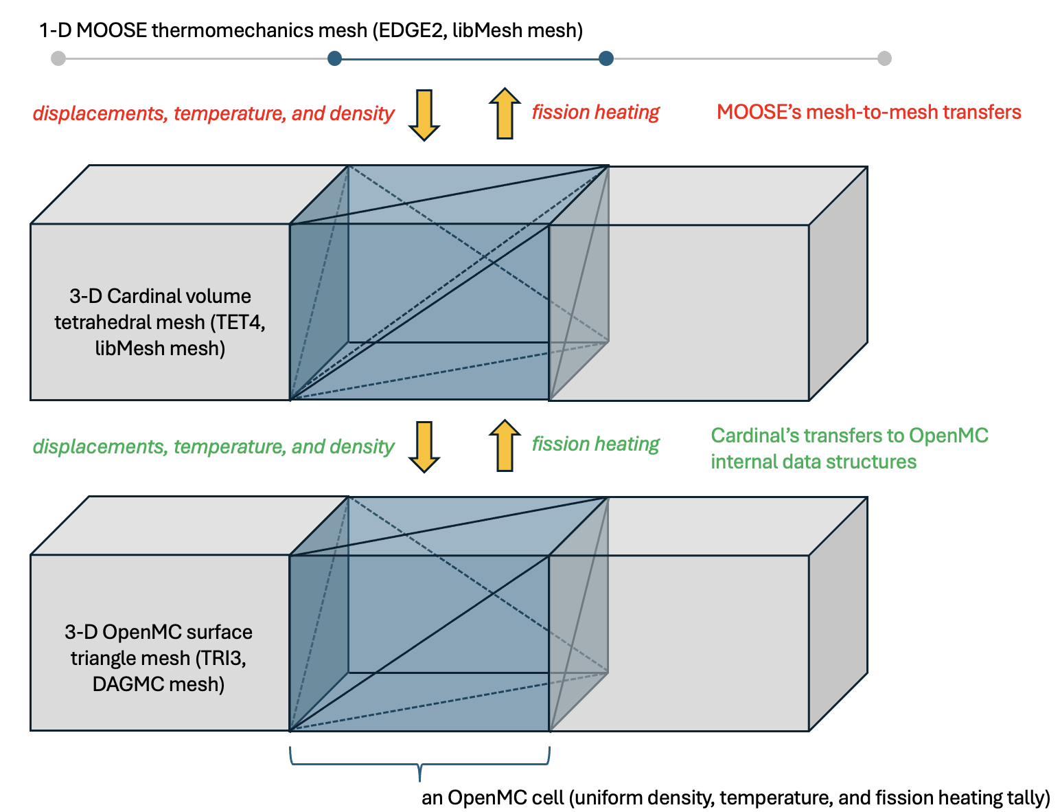
Figure 2: Data transfers between OpenMC and MOOSE and conceptual depiction of the different meshes used.

We show the input files for a coarse mesh here with more details on results convergence shown in the next section.

The OpenMC input files is as follows:

# This script creates the OpenMC model for the slab benchmark with temperature-dependent
# cross sections and uses DAGMC for geometry representation.

import openmc
import openmc.mgxs as mgxs
import numpy as np
import h5py

T0 = 293 # K
Tmax = 390 # K
Tmin = 290 # K
L0 = 100 # cm
L = 106.47 # cm
rho = 1.2 # g/cc
N_A = 6.022e23 # Avagadro's number
A = 180 # mass number for slab material
num_dens = rho*N_A/A
P = 1.0e22 # eV/s
q = 1e8 # eV
k0 = 1.25e19 # eV/(s-cm-K^2)
phi0 = 2.5e14 # 1/s-cm^2
s = 0.45 # Sigma_s/Sigma_t
f = 1.5 # nu Sigma_f/Sigma_t
nu = f/(1-s)
lam = 0.5*(1+np.sqrt(1+(16*q*q*phi0*phi0)/(P*P)))
Sig_t0 = np.sqrt(P/((lam-1)*k0*L))/(T0) # 1/cm
sig_t0 = Sig_t0/num_dens # cm^2
N = 20
infdim = 0.5

model = openmc.Model()

dagmc_univ = openmc.DAGMCUniverse(filename="slab20v.h5m")
model.geometry = openmc.Geometry(root=dagmc_univ)
cells = dagmc_univ.get_all_cells().values()

slab = openmc.Material(1, "slab")
slab.set_density('macro',1.)
slab.add_macroscopic('slab_xs')

model.materials = openmc.Materials([slab])
model.materials.cross_sections = 'one_group.h5'

groups = mgxs.EnergyGroups(group_edges=[0.0, 20.0e6])
NT = 100
temps = np.linspace(Tmin,Tmax,NT)
xsdata = openmc.XSdata('slab_xs', energy_groups=groups, temperatures=temps, num_delayed_groups=0)
xsdata.order = 0

for T in temps:
    Sig_t = (Sig_t0 * T0) / T
    Sig_s = s*Sig_t
    nu_Sig_f = f*Sig_t
    Sig_f = nu_Sig_f / nu
    Sig_a = Sig_f
    xsdata.set_total(np.array([Sig_t]),temperature=T)
    xsdata.set_scatter_matrix(np.array([[[Sig_s]]]),temperature=T)
    xsdata.set_absorption(np.array([Sig_a]),temperature=T)
    xsdata.set_fission(np.array([Sig_f]),temperature=T)
    xsdata.set_nu_fission(np.array([nu_Sig_f]),temperature=T)
    xsdata.set_kappa_fission(np.array([q*Sig_t]),temperature=T)

one_g_XS_file = openmc.MGXSLibrary(groups)
one_g_XS_file.add_xsdata(xsdata)
one_g_XS_file.export_to_hdf5('one_group.h5')

model.settings = openmc.Settings()
batches = 150
inactive = 50
particles = 50000
model.settings.energy_mode = 'multi-group'
model.settings.batches = batches
model.settings.inactive = inactive
model.settings.particles = particles
model.settings.output = {'tallies': True,'summary':False}

bounds = [-60, -infdim, -infdim, 60, infdim, infdim]
uniform_dist = openmc.stats.Box(bounds[:3], bounds[3:])
mu = openmc.stats.Discrete([0.0],[1.0])
phi = openmc.stats.Discrete([0,np.pi],[0.5,0.5])
bidirectional_x = openmc.stats.PolarAzimuthal(mu=mu,phi=phi)
model.settings.source = openmc.IndependentSource(space=uniform_dist,angle=bidirectional_x)
model.settings.temperature = {'default': (Tmin+Tmax)/2,
                        'method': 'interpolation',
                        'tolerance': 1,
                        'range': (Tmin, Tmax)}

model.export_to_model_xml()

The neutronics input file is as follows:

# Cardinal input file for slab benchmark OpenMC model to couple with thermomechanics

P = ${units 1.0e22 eV/s}
eV_to_J = ${units 1.602176634e-19 J/eV}
initial_temperature = ${units 293 K}

[Mesh<<<{"href": "../../syntax/Mesh/index.html"}>>>]
  [file]
    type = FileMeshGenerator<<<{"description": "Read a mesh from a file.", "href": "../../source/meshgenerators/FileMeshGenerator.html"}>>>
    file<<<{"description": "The filename to read."}>>> = slab20v.e
  []
[]

[GlobalParams<<<{"href": "../../syntax/GlobalParams/index.html"}>>>]
  displacements = 'disp_x disp_y disp_z'
  use_displaced_mesh = true
[]

[Variables<<<{"href": "../../syntax/Variables/index.html"}>>>]
  [disp_x]
  []
  [disp_y]
    initial_condition<<<{"description": "Specifies a constant initial condition for this variable"}>>> = 0.0
  []
  [disp_z]
    initial_condition<<<{"description": "Specifies a constant initial condition for this variable"}>>> = 0.0
  []
[]

[AuxVariables<<<{"href": "../../syntax/AuxVariables/index.html"}>>>]
  [bins]
    family<<<{"description": "Specifies the family of FE shape functions to use for this variable"}>>> = MONOMIAL
    order<<<{"description": "Specifies the order of the FE shape function to use for this variable (additional orders not listed are allowed)"}>>> = CONSTANT
  []
[]

[AuxKernels<<<{"href": "../../syntax/AuxKernels/index.html"}>>>]
  [bins]
    type = SkinnedBins<<<{"description": "Bins created by a skinner", "href": "../../source/auxkernels/SkinnedBins.html"}>>>
    variable<<<{"description": "The name of the variable that this object applies to"}>>> = bins
    skinner<<<{"description": "MOAB mesh skinner"}>>> = moab
  []
[]

[ICs<<<{"href": "../../syntax/Cardinal/ICs/index.html"}>>>]
  [temperature]
    type = FunctionIC<<<{"description": "An initial condition that uses a normal function of x, y, z to produce values (and optionally gradients) for a field variable.", "href": "../../source/ics/FunctionIC.html"}>>>
    variable<<<{"description": "The variable this initial condition is supposed to provide values for."}>>> = temperature
    function<<<{"description": "The initial condition function."}>>> = ${initial_temperature}
  []
[]

[Problem<<<{"href": "../../syntax/Problem/index.html"}>>>]
  type = OpenMCCellAverageProblem
  verbose = true
  source_rate_normalization = 'kappa_fission'
  inactive_batches = 150
  batches = 300
  particles = 100000
  power = '${fparse P*eV_to_J}'
  cell_level = 0
  temperature_variables = 'temperature'
  temperature_blocks = '1 2 3 4 5 6 7 8 9 10 11 12 13 14 15 16 17 18 19 20'
  volume_calculation = vol
  skinner = moab
  [Tallies<<<{"href": "../../syntax/Problem/Tallies/index.html"}>>>]
    [kappa_fission]
      type = CellTally<<<{"description": "A class which implements distributed cell tallies.", "href": "../../source/tallies/CellTally.html"}>>>
      estimator<<<{"description": "Type of tally estimator to use in OpenMC"}>>> = collision
      block<<<{"description": "Subdomains for which to add tallies in OpenMC. If not provided, tallies will be applied over the entire domain corresponding to the [Mesh] block."}>>> = '1 2 3 4 5 6 7 8 9 10 11 12 13 14 15 16 17 18 19 20'
      name<<<{"description": "Auxiliary variable name(s) to use for OpenMC tallies. If not specified, defaults to the names of the scores"}>>> = kappa_fission
      output<<<{"description": "UNRELAXED field(s) to output from OpenMC for each tally score. unrelaxed_tally_std_dev will write the standard deviation of each tally into auxiliary variables named *_std_dev. unrelaxed_tally_rel_error will write the relative standard deviation (unrelaxed_tally_std_dev / unrelaxed_tally) of each tally into auxiliary variables named *_rel_error. unrelaxed_tally will write the raw unrelaxed tally into auxiliary variables named *_raw (replace * with 'name')."}>>> = unrelaxed_tally_std_dev
    []
    [flux]
      type = CellTally<<<{"description": "A class which implements distributed cell tallies.", "href": "../../source/tallies/CellTally.html"}>>>
      estimator<<<{"description": "Type of tally estimator to use in OpenMC"}>>> = collision
      block<<<{"description": "Subdomains for which to add tallies in OpenMC. If not provided, tallies will be applied over the entire domain corresponding to the [Mesh] block."}>>> = '1 2 3 4 5 6 7 8 9 10 11 12 13 14 15 16 17 18 19 20'
      score<<<{"description": "Score(s) to use in the OpenMC tallies. If not specified, defaults to 'kappa_fission'"}>>> = flux
      output<<<{"description": "UNRELAXED field(s) to output from OpenMC for each tally score. unrelaxed_tally_std_dev will write the standard deviation of each tally into auxiliary variables named *_std_dev. unrelaxed_tally_rel_error will write the relative standard deviation (unrelaxed_tally_std_dev / unrelaxed_tally) of each tally into auxiliary variables named *_rel_error. unrelaxed_tally will write the raw unrelaxed tally into auxiliary variables named *_raw (replace * with 'name')."}>>> = unrelaxed_tally_std_dev
    []
  []
[]

[Executioner<<<{"href": "../../syntax/Executioner/index.html"}>>>]
  type = Transient
  start_time = 0.0
  end_time = 1e5
  dt = 500
[]

[MultiApps<<<{"href": "../../syntax/MultiApps/index.html"}>>>]
  [solid]
    type = TransientMultiApp<<<{"description": "MultiApp for performing coupled simulations with the parent and sub-application both progressing in time.", "href": "../../source/multiapps/TransientMultiApp.html"}>>>
    input_files<<<{"description": "The input file for each App.  If this parameter only contains one input file it will be used for all of the Apps.  When using 'positions_from_file' it is also admissable to provide one input_file per file."}>>> = 'solid.i'
    execute_on<<<{"description": "The list of flag(s) indicating when this object should be executed. For a description of each flag, see https://mooseframework.inl.gov/source/interfaces/SetupInterface.html."}>>> = timestep_end
  []
[]

[Transfers<<<{"href": "../../syntax/Transfers/index.html"}>>>]
  [kappa_fission_to_solid]
    type = MultiAppGeneralFieldShapeEvaluationTransfer<<<{"description": "Transfers field data at the MultiApp position using the finite element shape functions from the origin application.", "href": "../../source/transfers/MultiAppGeneralFieldShapeEvaluationTransfer.html"}>>>
    to_multi_app<<<{"description": "The name of the MultiApp to transfer the data to"}>>> = solid
    variable<<<{"description": "The auxiliary variable to store the transferred values in."}>>> = kappa_fission
    source_variable<<<{"description": "The variable to transfer from."}>>> = kappa_fission
    from_postprocessors_to_be_preserved<<<{"description": "The name of the Postprocessor in the from-app to evaluate an adjusting factor."}>>> = heat_source
    to_postprocessors_to_be_preserved<<<{"description": "The name of the Postprocessor in the to-app to evaluate an adjusting factor."}>>> = source_integral
    execute_on<<<{"description": "The list of flag(s) indicating when this object should be executed. For a description of each flag, see https://mooseframework.inl.gov/source/interfaces/SetupInterface.html."}>>> = timestep_end
    displaced_source_mesh<<<{"description": "Whether or not to use the displaced mesh for the source mesh."}>>> = true
    displaced_target_mesh<<<{"description": "Whether or not to use the displaced mesh for the target mesh."}>>> = true
  []
  [temperature_from_solid]
    type = MultiAppGeneralFieldNearestLocationTransfer<<<{"description": "Transfers field data at the MultiApp position by finding the value at the nearest neighbor(s) in the origin application.", "href": "../../source/transfers/MultiAppGeneralFieldNearestLocationTransfer.html"}>>>
    from_multi_app<<<{"description": "The name of the MultiApp to receive data from"}>>> = solid
    variable<<<{"description": "The auxiliary variable to store the transferred values in."}>>> = temperature
    source_variable<<<{"description": "The variable to transfer from."}>>> = temperature_praux
    execute_on<<<{"description": "The list of flag(s) indicating when this object should be executed. For a description of each flag, see https://mooseframework.inl.gov/source/interfaces/SetupInterface.html."}>>> = timestep_end
    displaced_source_mesh<<<{"description": "Whether or not to use the displaced mesh for the source mesh."}>>> = true
    displaced_target_mesh<<<{"description": "Whether or not to use the displaced mesh for the target mesh."}>>> = true
  []
  [dispx]
    type = MultiAppGeneralFieldNearestLocationTransfer<<<{"description": "Transfers field data at the MultiApp position by finding the value at the nearest neighbor(s) in the origin application.", "href": "../../source/transfers/MultiAppGeneralFieldNearestLocationTransfer.html"}>>>
    source_variable<<<{"description": "The variable to transfer from."}>>> = disp_praux
    variable<<<{"description": "The auxiliary variable to store the transferred values in."}>>> = disp_x
    from_multi_app<<<{"description": "The name of the MultiApp to receive data from"}>>> = solid
    displaced_source_mesh<<<{"description": "Whether or not to use the displaced mesh for the source mesh."}>>> = true
    displaced_target_mesh<<<{"description": "Whether or not to use the displaced mesh for the target mesh."}>>> = true
  []
[]

[Outputs<<<{"href": "../../syntax/Outputs/index.html"}>>>]
  exodus<<<{"description": "Output the results using the default settings for Exodus output."}>>> = false
  csv<<<{"description": "Output the scalar variable and postprocessors to a *.csv file using the default CSV output."}>>> = true
[]

[Postprocessors<<<{"href": "../../syntax/Postprocessors/index.html"}>>>]
  [heat_source]
    type = ElementIntegralVariablePostprocessor<<<{"description": "Computes a volume integral of the specified variable", "href": "../../source/postprocessors/ElementIntegralVariablePostprocessor.html"}>>>
    variable<<<{"description": "The name of the variable that this object operates on"}>>> = kappa_fission
    execute_on<<<{"description": "The list of flag(s) indicating when this object should be executed. For a description of each flag, see https://mooseframework.inl.gov/source/interfaces/SetupInterface.html."}>>> = 'transfer initial timestep_end'
  []
  [k]
    type = KEigenvalue<<<{"description": "k eigenvalue computed by OpenMC", "href": "../../source/postprocessors/KEigenvalue.html"}>>>
  []
  [k_std_dev]
    type = KEigenvalue<<<{"description": "k eigenvalue computed by OpenMC", "href": "../../source/postprocessors/KEigenvalue.html"}>>>
    output<<<{"description": "The value to output. Options are $k_{eff}$ (mean), the standard deviation of $k_{eff}$ (std_dev), or the relative error of $k_{eff}$ (rel_err)."}>>> = 'std_dev'
  []
[]

[VectorPostprocessors<<<{"href": "../../syntax/VectorPostprocessors/index.html"}>>>]
  [temperature]
    type = ElementValueSampler<<<{"description": "Samples values of variables on elements.", "href": "../../source/vectorpostprocessors/ElementValueSampler.html"}>>>
    variable<<<{"description": "The names of the variables that this VectorPostprocessor operates on"}>>> = 'temperature'
    sort_by<<<{"description": "What to sort the samples by. Options include 'x', 'y', 'z', 'id', and the name of any of the sampled quantities (which each create a vector of the same name)."}>>> = x
    execute_on<<<{"description": "The list of flag(s) indicating when this object should be executed. For a description of each flag, see https://mooseframework.inl.gov/source/interfaces/SetupInterface.html."}>>> = 'FINAL'
  []
[]

[UserObjects<<<{"href": "../../syntax/UserObjects/index.html"}>>>]
  [vol]
    type = OpenMCVolumeCalculation<<<{"description": "Stochastic volume calculation of the OpenMC cells which map to MOOSE", "href": "../../source/userobjects/OpenMCVolumeCalculation.html"}>>>
    n_samples<<<{"description": "Number of samples to use for the stochastic volume calculation"}>>> = 200000
  []
  [moab]
    type = MoabSkinner<<<{"description": "Re-generate the OpenMC geometry on-the-fly according to changes in the mesh geometry and/or contours in temperature and density", "href": "../../source/userobjects/MoabSkinner.html"}>>>
    execute_on<<<{"description": "The list of flag(s) indicating when this object should be executed. For a description of each flag, see https://mooseframework.inl.gov/source/interfaces/SetupInterface.html."}>>> = 'timestep_begin'
    verbose<<<{"description": "Whether to print diagnostic information"}>>> = true
    temperature<<<{"description": "Temperature variable by which to bin elements"}>>> = temperature
    n_temperature_bins<<<{"description": "Number of temperature bins"}>>> = 1.0
    temperature_min<<<{"description": "Lower bound of temperature bins"}>>> = 0.0
    temperature_max<<<{"description": "Upper bound of temperature bins"}>>> = 1000
    build_graveyard<<<{"description": "Whether to build a graveyard around the geometry"}>>> = true
    graveyard_scale_inner<<<{"description": "Multiplier on mesh bounding box to form inner graveyard surface"}>>> = 1.5
    graveyard_scale_outer<<<{"description": "Multiplier on mesh bounding box to form outer graveyard surface"}>>> = 1.6
  []
[]

The thermomechanics input file is as follows:

# MOOSE Thermomechanics model input file for the slab benchmark problem

T0 = ${units 293 K}
L0 = ${units 100 cm}
L = ${units 106.47 cm}
P = ${units 1.0e22 eV/s}
q = ${units 1e8 eV}
k0 = ${units 1.25e19 eV/s/cm/K^2} # k(T) = k0 T(x)
phi0 = ${units 2.5e14 1/s/cm^2} # (flux at the origin)
eV_to_J = ${units 1.602176634e-19 J/eV}
lam = '${fparse 0.5*(1+sqrt(1+(16*q*q*phi0*phi0)/(P*P)))}' # eigenvalue solution
h = '${fparse 1/(sqrt(L*(lam-1)/(k0*P)) - (2*T0)/(P))*eV_to_J }' # W/cm^2-K

E = ${units 1e6 N/m^2}
nu = 0.0
rho = ${units 20 g/cm^3}
c_p = ${units 0.3 J/g/K}

[Mesh<<<{"href": "../../syntax/Mesh/index.html"}>>>]
  [generated]
    type = GeneratedMeshGenerator<<<{"description": "Create a line, square, or cube mesh with uniformly spaced or biased elements.", "href": "../../source/meshgenerators/GeneratedMeshGenerator.html"}>>>
    dim<<<{"description": "The dimension of the mesh to be generated"}>>> = 1
    nx<<<{"description": "Number of elements in the X direction"}>>> = 20
    xmin<<<{"description": "Lower X Coordinate of the generated mesh"}>>> = -50
    xmax<<<{"description": "Upper X Coordinate of the generated mesh"}>>> = 50
  []
  [pin]
    type = ExtraNodesetGenerator<<<{"description": "Creates a new node set and a new boundary made with the nodes the user provides.", "href": "../../source/meshgenerators/ExtraNodesetGenerator.html"}>>>
    input<<<{"description": "The mesh we want to modify"}>>> = generated
    new_boundary<<<{"description": "The names of the boundaries to create"}>>> = pin
    coord<<<{"description": "The nodes with coordinates you want to be in the nodeset. Separate multple coords with ';' (Either this parameter or \"nodes\" must be supplied)."}>>> = '0 0 0'
  []
[]

[Problem<<<{"href": "../../syntax/Problem/index.html"}>>>]
  type = ReferenceResidualProblem
  extra_tag_vectors = 'ref'
  reference_vector = 'ref'
[]

[GlobalParams<<<{"href": "../../syntax/GlobalParams/index.html"}>>>]
  displacements = 'disp_x'
  use_displaced_mesh = true
[]

[Variables<<<{"href": "../../syntax/Variables/index.html"}>>>]
  [temperature]
  []
  [disp_x]
  []
[]

[Physics<<<{"href": "../../syntax/Physics/index.html"}>>>]
  [SolidMechanics<<<{"href": "../../syntax/Physics/SolidMechanics/index.html"}>>>]
    [QuasiStatic<<<{"href": "../../syntax/Physics/SolidMechanics/QuasiStatic/index.html"}>>>]
      [block1]
        strain<<<{"description": "Strain formulation"}>>> = FINITE
        add_variables<<<{"description": "Add the displacement variables"}>>> = true
        eigenstrain_names<<<{"description": "List of eigenstrains to be applied in this strain calculation"}>>> = eigenstrain
        generate_output<<<{"description": "Add scalar quantity output for stress and/or strain"}>>> = 'strain_xx'
        temperature<<<{"description": "The temperature"}>>> = temperature
      []
    []
  []
[]

[ICs<<<{"href": "../../syntax/Cardinal/ICs/index.html"}>>>]
  [temperature]
    type = FunctionIC<<<{"description": "An initial condition that uses a normal function of x, y, z to produce values (and optionally gradients) for a field variable.", "href": "../../source/ics/FunctionIC.html"}>>>
    variable<<<{"description": "The variable this initial condition is supposed to provide values for."}>>> = temperature
    function<<<{"description": "The initial condition function."}>>> = ${T0}
  []
[]

[Kernels<<<{"href": "../../syntax/Kernels/index.html"}>>>]
  [heat_conduction]
    type = HeatConduction<<<{"description": "Diffusive heat conduction term $-\\nabla\\cdot(k\\nabla T)$ of the thermal energy conservation equation", "href": "../../source/kernels/HeatConduction.html"}>>>
    variable<<<{"description": "The name of the variable that this residual object operates on"}>>> = temperature
  []
  [kappa_fission]
    type = CoupledForce<<<{"description": "Implements a source term proportional to the value of a coupled variable. Weak form: $(\\psi_i, -\\sigma v)$.", "href": "../../source/kernels/CoupledForce.html"}>>>
    variable<<<{"description": "The name of the variable that this residual object operates on"}>>> = temperature
    v<<<{"description": "The coupled variable which provides the force"}>>> = kappa_fission
  []
  [dt]
    type = HeatConductionTimeDerivative<<<{"description": "Time derivative term $\\rho c_p \\frac{\\partial T}{\\partial t}$ of the thermal energy conservation equation.", "href": "../../source/kernels/HeatConductionTimeDerivative.html"}>>>
    variable<<<{"description": "The name of the variable that this residual object operates on"}>>> = temperature
  []
[]

[AuxVariables<<<{"href": "../../syntax/AuxVariables/index.html"}>>>]
  [kappa_fission]
    family<<<{"description": "Specifies the family of FE shape functions to use for this variable"}>>> = MONOMIAL
    order<<<{"description": "Specifies the order of the FE shape function to use for this variable (additional orders not listed are allowed)"}>>> = CONSTANT
    initial_condition<<<{"description": "Specifies a constant initial condition for this variable"}>>> = '${fparse P*eV_to_J/L0 }'
  []
  [temperature_praux]
    family<<<{"description": "Specifies the family of FE shape functions to use for this variable"}>>> = MONOMIAL
    order<<<{"description": "Specifies the order of the FE shape function to use for this variable (additional orders not listed are allowed)"}>>> = CONSTANT
  []
  [disp_praux]
  []
[]

[AuxKernels<<<{"href": "../../syntax/AuxKernels/index.html"}>>>]
  [temperature_projection]
    type = ProjectionAux<<<{"description": "Returns the specified variable as an auxiliary variable with a projection of the source variable. If they are the same type, this amounts to a simple copy.", "href": "../../source/auxkernels/ProjectionAux.html"}>>>
    variable<<<{"description": "The name of the variable that this object applies to"}>>> = temperature_praux
    v<<<{"description": "Variable to take the value of."}>>> = temperature
  []
  [disp_projection]
    type = ProjectionAux<<<{"description": "Returns the specified variable as an auxiliary variable with a projection of the source variable. If they are the same type, this amounts to a simple copy.", "href": "../../source/auxkernels/ProjectionAux.html"}>>>
    variable<<<{"description": "The name of the variable that this object applies to"}>>> = disp_praux
    v<<<{"description": "Variable to take the value of."}>>> = disp_x
  []
[]

[Materials<<<{"href": "../../syntax/Materials/index.html"}>>>]
  [thermal_parameters]
    type = HeatConductionMaterial<<<{"description": "General-purpose material model for heat conduction", "href": "../../source/materials/HeatConductionMaterial.html"}>>>
    temperature<<<{"description": "Coupled Temperature"}>>> = temperature
    thermal_conductivity_temperature_function<<<{"description": "Thermal conductivity as a function of temperature."}>>> = conductivity
    specific_heat<<<{"description": "The specific heat value"}>>> = ${c_p}
  []
  [density]
    type = ParsedMaterial<<<{"description": "Parsed expression Material.", "href": "../../source/materials/ParsedMaterial.html"}>>>
    property_name<<<{"description": "Name of the parsed material property"}>>> = density
    expression<<<{"description": "Parsed function (see FParser) expression for the parsed material"}>>> = ${rho}
  []
  [elasticity_tensor]
    type = ComputeIsotropicElasticityTensor<<<{"description": "Compute a constant isotropic elasticity tensor.", "href": "../../source/materials/ComputeIsotropicElasticityTensor.html"}>>>
    youngs_modulus<<<{"description": "Young's modulus of the material."}>>> = ${E}
    poissons_ratio<<<{"description": "Poisson's ratio for the material."}>>> = ${nu}
  []
  [stress]
    type = ComputeFiniteStrainElasticStress<<<{"description": "Compute stress using elasticity for finite strains", "href": "../../source/materials/ComputeFiniteStrainElasticStress.html"}>>>
  []
  [thermal_expansion_strain]
    type = ComputeMeanThermalExpansionFunctionEigenstrain<<<{"description": "Computes eigenstrain due to thermal expansion using a function that describes the mean thermal expansion as a function of temperature", "href": "../../source/materials/ComputeMeanThermalExpansionFunctionEigenstrain.html"}>>>
    stress_free_temperature<<<{"description": "Reference temperature at which there is no thermal expansion for thermal eigenstrain calculation"}>>> = ${T0}
    thermal_expansion_function_reference_temperature<<<{"description": "Reference temperature for thermal_exansion_function (IMPORTANT: this is different in general from the stress_free_temperature)"}>>> = ${T0}
    thermal_expansion_function<<<{"description": "Function describing the mean thermal expansion as a function of temperature"}>>> = cte_func_mean
    temperature<<<{"description": "Coupled temperature"}>>> = temperature
    eigenstrain_name<<<{"description": "Material property name for the eigenstrain tensor computed by this model. IMPORTANT: The name of this property must also be provided to the strain calculator."}>>> = eigenstrain
  []
[]

[BCs<<<{"href": "../../syntax/BCs/index.html"}>>>]
  [sides_convective_BC]
    type = ConvectiveFluxFunction<<<{"description": "Determines boundary value by fluid heat transfer coefficient and far-field temperature", "href": "../../source/bcs/ConvectiveFluxFunction.html"}>>>
    T_infinity<<<{"description": "Function describing far-field temperature"}>>> = ${T0}
    variable<<<{"description": "The name of the variable that this residual object operates on"}>>> = temperature
    boundary<<<{"description": "The list of boundary IDs from the mesh where this object applies"}>>> = 'left right'
    coefficient<<<{"description": "Function describing heat transfer coefficient"}>>> = ${h}
  []
  [pin_x]
    type = DirichletBC<<<{"description": "Imposes the essential boundary condition $u=g$, where $g$ is a constant, controllable value.", "href": "../../source/bcs/DirichletBC.html"}>>>
    variable<<<{"description": "The name of the variable that this residual object operates on"}>>> = disp_x
    boundary<<<{"description": "The list of boundary IDs from the mesh where this object applies"}>>> = 'pin'
    value<<<{"description": "Value of the BC"}>>> = 0.0
  []
[]

[Functions<<<{"href": "../../syntax/Functions/index.html"}>>>]
  [conductivity]
    type = ParsedFunction<<<{"description": "Function created by parsing a string", "href": "../../source/functions/MooseParsedFunction.html"}>>>
    expression<<<{"description": "The user defined function."}>>> = '${fparse k0*eV_to_J} * t'
  []
  [cte_func_mean]
    type = ParsedFunction<<<{"description": "Function created by parsing a string", "href": "../../source/functions/MooseParsedFunction.html"}>>>
    expression<<<{"description": "The user defined function."}>>> = '1 / (2*sqrt(${T0}*t))'
  []
[]

[Executioner<<<{"href": "../../syntax/Executioner/index.html"}>>>]
  type = Transient
  solve_type = 'PJFNK'
  verbose = true
  nl_abs_tol = 1e-9
  nl_rel_tol = 1e-9
  petsc_options = '-ksp_snes_ew'
  petsc_options_iname = '-pc_type -pc_factor_mat_solver_package'
  petsc_options_value = 'lu       superlu_dist'
  snesmf_reuse_base = false
  line_search = 'none'
  nl_max_its = 100
  [TimeStepper<<<{"href": "../../syntax/Executioner/TimeStepper/index.html"}>>>]
    type = IterationAdaptiveDT
    dt = 1e-1
    optimal_iterations = 10
    growth_factor = 1.25
    cutback_factor = 0.8
  []
[]

[Preconditioning<<<{"href": "../../syntax/Preconditioning/index.html"}>>>]
  [smp]
    type = SMP<<<{"description": "Single matrix preconditioner (SMP) builds a preconditioner using user defined off-diagonal parts of the Jacobian.", "href": "../../source/preconditioners/SingleMatrixPreconditioner.html"}>>>
    full<<<{"description": "Set to true if you want the full set of couplings between variables simply for convenience so you don't have to set every off_diag_row and off_diag_column combination."}>>> = true
  []
[]

[Outputs<<<{"href": "../../syntax/Outputs/index.html"}>>>]
  exodus<<<{"description": "Output the results using the default settings for Exodus output."}>>> = false
  csv<<<{"description": "Output the scalar variable and postprocessors to a *.csv file using the default CSV output."}>>> = true
[]

[Postprocessors<<<{"href": "../../syntax/Postprocessors/index.html"}>>>]
  [source_integral]
    type = ElementIntegralVariablePostprocessor<<<{"description": "Computes a volume integral of the specified variable", "href": "../../source/postprocessors/ElementIntegralVariablePostprocessor.html"}>>>
    variable<<<{"description": "The name of the variable that this object operates on"}>>> = kappa_fission
    execute_on<<<{"description": "The list of flag(s) indicating when this object should be executed. For a description of each flag, see https://mooseframework.inl.gov/source/interfaces/SetupInterface.html."}>>> = 'transfer initial timestep_end'
  []
  [strain_xx]
    type = ElementAverageValue<<<{"description": "Computes the volumetric average of a variable", "href": "../../source/postprocessors/ElementAverageValue.html"}>>>
    variable<<<{"description": "The name of the variable that this object operates on"}>>> = strain_xx
  []
  [total_length]
    type = FunctionElementIntegral<<<{"description": "Integrates a function over elements", "href": "../../source/postprocessors/FunctionElementIntegral.html"}>>>
    function<<<{"description": "Name of function to integrate"}>>> = 1
    execute_on<<<{"description": "The list of flag(s) indicating when this object should be executed. For a description of each flag, see https://mooseframework.inl.gov/source/interfaces/SetupInterface.html."}>>> = 'TIMESTEP_BEGIN LINEAR TIMESTEP_END'
  []
[]

It is important to note that incremental (hypoelastic) formulations of finite strain behavior inherently introduce inaccuracies arising from the time integration error. This limitation is inherent to this formulation and therefore exists in the MOOSE implementation and the implementations of other major commercial codes. The magnitude of these errors grows with increasing strain, so this typically becomes a practical issue only for very large strains, for which hyperelastic models are more appropriate (Belytschko et al., 2003).

The main sources of error in this coupled model are: (i) the statistical error from use of finite particles in OpenMC; (ii) the user-input cross-section data, which is defined with 1 K $var element = document.getElementById("moose-equation-3b79fbe7-5fda-4f27-917c-e7e1226b0f27");katex.render("\\Delta", element, {displayMode:false,throwOnError:false});$ T spacings used in all cases while taking the nearest temperature point cross section; and (iii) discretization error from a finite spatial mesh in both OpenMC (temperature feedback resolution) and MOOSE thermomechanics. Additional sources of error are present, but anticipated to be negligible due to the use of fine settings for these simulation parameters: (i) finite Picard iterations, and (ii) nonzero nonlinear tolerances in the MOOSE thermomechanics model.

Results

We see the heating result in Figure 3 compared against the analytic solution, as well as flux and temperature solutions in Figure 4 and Figure 5. Figures are only included for $var element = document.getElementById("moose-equation-464bd4b1-a251-47d1-874a-b8bcd3265f79");katex.render("P=1.0 \\times 10^{22}", element, {displayMode:false,throwOnError:false});$ eV/s and on a fine mesh where the number of OpenMC and mesh elements is $var element = document.getElementById("moose-equation-1ad3deed-44ba-4652-b500-c4518cb77039");katex.render("N = 100", element, {displayMode:false,throwOnError:false});$ , since all results have a similar shape. 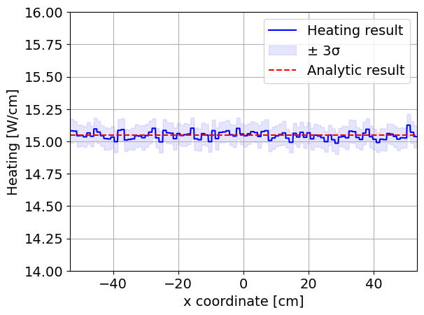Both the heating and flux tally everywhere agree with the analytic solution within 3 $var element = document.getElementById("moose-equation-3dff33e6-b167-4191-b5f8-3fe07488caf6");katex.render("\\sigma", element, {displayMode:false,throwOnError:false});$ .

Figure 3: Heating result from OpenMC for N = 100 mesh elements compared against the analytic solution.

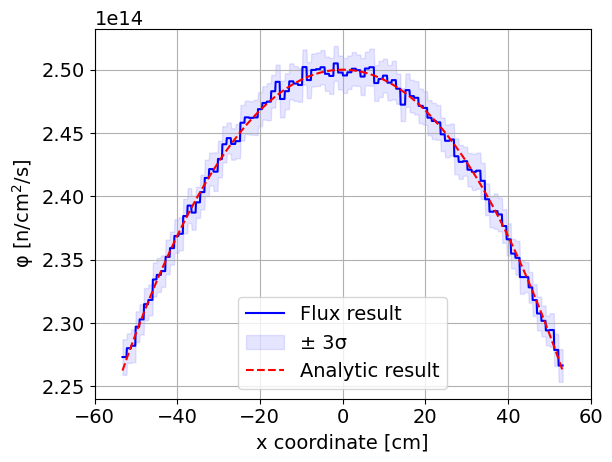
Figure 4: Flux result from OpenMC for N = 100 mesh elements compared against the analytic solution.

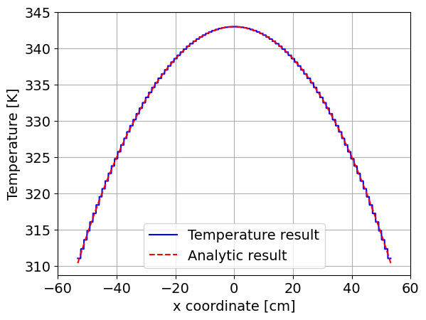
Figure 5: Temperature result from MOOSE for N = 100 mesh elements compared against the analytic solution.

Table 2 shows results convergence with mesh refinement.

Table 2: Results and corresponding errors with different mesh sizes (Eltawila et al., 2026).

Resolution	Heated length (cm)	Error (μm)	$var element = document.getElementById("moose-equation-1307789f-cd37-4236-8b67-d53a63974463");katex.render("k_{\\text{eff}}", element, {displayMode:false,throwOnError:false});$	Error (pcm)
Analytic solution	106.47	–	0.29557	–
5	106.3298	-1402	0.29608 ± 0.00001	51 ± 1
10	106.4382	-318	0.29619 ± 0.00001	62 ± 1
20	106.4671	-29	0.29557 ± 0.00001	0 ± 1
50	106.4730	30	0.29536 ± 0.00001	-21 ± 1
100	106.4745	45	0.29549 ± 0.00001	-8 ± 1
200	106.4748	48	0.29556 ± 0.00001	-1 ± 1

In Figure 6 and Figure 7, convergence of flux and temperature relative L $var element = document.getElementById("moose-equation-82b2da32-d3c4-4177-91cd-64671eaae7ab");katex.render("^2", element, {displayMode:false,throwOnError:false});$ norms, defined as

$var element = document.getElementById("moose-equation-9cdd7902-8482-4619-afca-b3f6abd12a7d");katex.render(" \\varepsilon_\\phi=\\frac{||\\phi_a-\\phi_{sln.}||_2}{||\\phi_a||_2}", element, {displayMode:true,throwOnError:false});$

and

$var element = document.getElementById("moose-equation-7c27bb00-a1aa-4aec-842d-d4ac8d0cafea");katex.render(" \\varepsilon_T=\\frac{||T_a-T_{sln.}||_2}{||T_a||_2}", element, {displayMode:true,throwOnError:false});$

where $var element = document.getElementById("moose-equation-c5b01c1a-65e7-4612-a5f7-768f4c1dbbfc");katex.render("\\phi_a", element, {displayMode:false,throwOnError:false});$ is the analytic flux solution, $var element = document.getElementById("moose-equation-edcd183a-7da1-4ae2-9254-1274494dbd0d");katex.render("\\phi_{sln.}", element, {displayMode:false,throwOnError:false});$ is the Cardinal flux solution, $var element = document.getElementById("moose-equation-7f8d8b4d-2305-489e-a637-aac7987ef1e2");katex.render("T_a", element, {displayMode:false,throwOnError:false});$ is the analytic temperature solution, and $var element = document.getElementById("moose-equation-5ef59aa4-4f76-49ff-a85e-b1cfb541c79e");katex.render("T_{sln.}", element, {displayMode:false,throwOnError:false});$ is the Cardinal temperature solution.

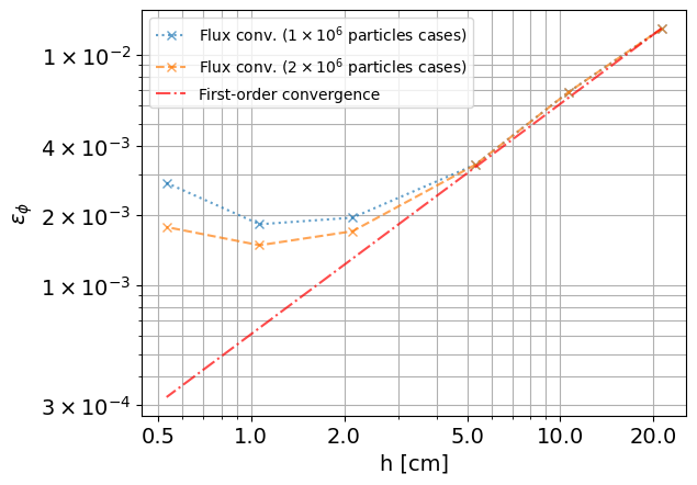
Convergence of flux relative L$^2$ norm.

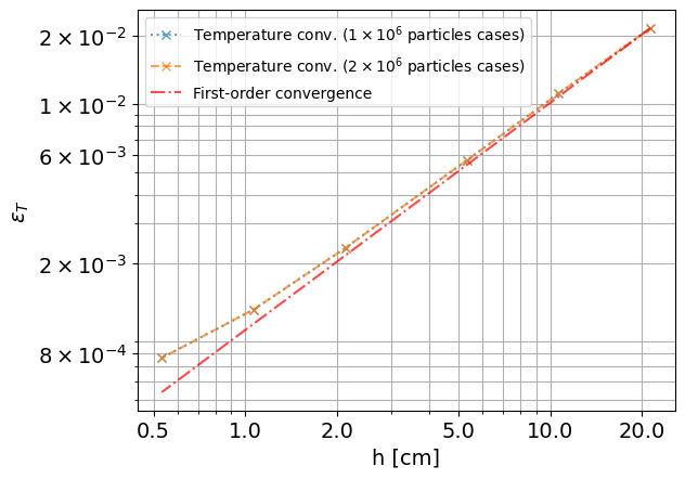
Figure 6: Convergence of flux relative L $var element = document.getElementById("moose-equation-1f823df1-8239-4af0-a518-a0c59ad79486");katex.render("^2", element, {displayMode:false,throwOnError:false});$ norm.

Convergence of temperature relative L$^2$ norm.

Figure 7: Convergence of temperature relative L $var element = document.getElementById("moose-equation-6ef76214-3fe8-43b4-b6d0-5ec2b82a067f");katex.render("^2", element, {displayMode:false,throwOnError:false});$ norm.

A first-order convergence of the temperature is achieved with mesh refinement, while the flux starts to converge following a first-order trend then stagnates where other error components dominate as discussed earlier. The stochastic noise error influence is highlighted by keeping the number of particles constant for each line, where we see further convergence when there is less stochastic noise.

We hypothesize that the observed first-order convergence arises from the use of cell tallies in OpenMC, where heating results are tallied as constant monomials. This may be limiting the convergence rate of the coupled solve.

More details and discussion can be found in Eltawila et al. (2026).

References

Ted Belytschko, Wing Kam Liu, and Brian Moran. Nonlinear Finite Elements for Continua and Structures. John Wiley & Sons, West Sussex, England, 2003.

BibTeX

@book{belytschko2003,
    author = "Belytschko, Ted and Liu, Wing Kam and Moran, Brian",
    title = "{N}onlinear {F}inite {E}lements for {C}ontinua and {S}tructures",
    year = "2003",
    publisher = "John Wiley \\& Sons, West Sussex, England"
}

RIS

TY  - BOOK
AU  - Belytschko, Ted
AU  - Liu, Wing Kam
AU  - Moran, Brian
TI  - Nonlinear Finite Elements for Continua and Structures
PY  - 2003
PB  - John Wiley & Sons, West Sussex, England
ER  -

Plain Text

Ted Belytschko, Wing Kam Liu, and Brian Moran. Nonlinear Finite Elements for Continua and Structures. John Wiley & Sons, West Sussex, England, 2003.

Mahmoud Eltawila, Pierre-Clément A. Simon, Guillaume L. Giudicelli, Helen Brooks, Nicholas Wozniak, and April J. Novak. Thermomechanics coupling to Monte Carlo particle transport on unstructured mesh geometries using Cardinal. Annals of Nuclear Energy, 229:112068, 2026. URL: https://www.sciencedirect.com/science/article/pii/S0306454925008850, doi:https://doi.org/10.1016/j.anucene.2025.112068.

BibTeX

@article{ELTAWILA2026112068,
    author = "Eltawila, Mahmoud and Simon, Pierre-Clément A. and Giudicelli, Guillaume L. and Brooks, Helen and Wozniak, Nicholas and Novak, April J.",
    title = "{Thermomechanics coupling to Monte Carlo particle transport on unstructured mesh geometries using Cardinal}",
    journal = "Annals of Nuclear Energy",
    volume = "229",
    pages = "112068",
    year = "2026",
    issn = "0306-4549",
    doi = "https://doi.org/10.1016/j.anucene.2025.112068",
    url = "https://www.sciencedirect.com/science/article/pii/S0306454925008850"
}

RIS

TY  - JOUR
AU  - Eltawila, Mahmoud
AU  - Simon, Pierre-Clément A.
AU  - Giudicelli, Guillaume L.
AU  - Brooks, Helen
AU  - Wozniak, Nicholas
AU  - Novak, April J.
TI  - Thermomechanics coupling to Monte Carlo particle transport on unstructured mesh geometries using Cardinal
JO  - Annals of Nuclear Energy
PY  - 2026
VL  - 229
DO  - https://doi.org/10.1016/j.anucene.2025.112068
UR  - https://www.sciencedirect.com/science/article/pii/S0306454925008850
SP  - 112068
ER  -

Plain Text

Mahmoud Eltawila, Pierre-Clément A. Simon, Guillaume L. Giudicelli, Helen Brooks, Nicholas Wozniak, and April J. Novak. Thermomechanics coupling to Monte Carlo particle transport on unstructured mesh geometries using Cardinal. Annals of Nuclear Energy, 229:112068, 2026. URL: https://www.sciencedirect.com/science/article/pii/S0306454925008850, doi:https://doi.org/10.1016/j.anucene.2025.112068.

D. P. Griesheimer and G. Kooreman. Analytical benchmark solution for 1-D neutron transport coupled with thermal conduction and material expansion. In Proceedings of PHYSOR, 697–706. ANS, 07 2022.

BibTeX

@inproceedings{griesheimer2022analytical,
    author = "Griesheimer, D. P. and Kooreman, G.",
    title = "Analytical benchmark solution for {1-D} neutron transport coupled with thermal conduction and material expansion",
    place = "United States",
    organization = "ANS",
    year = "2022",
    month = "07",
    booktitle = "Proceedings of PHYSOR",
    pages = "697-706"
}

RIS

TY  - CPAPER
AU  - Griesheimer, D. P.
AU  - Kooreman, G.
TI  - Analytical benchmark solution for 1-D neutron transport coupled with thermal conduction and material expansion
T2  - Proceedings of PHYSOR
PY  - 2022
SP  - 697
EP  - 706
ER  -

Plain Text

D. P. Griesheimer and G. Kooreman. Analytical benchmark solution for 1-D neutron transport coupled with thermal conduction and material expansion. In Proceedings of PHYSOR, 697-706. ANS, 07 2022.

(test/tests/neutronics/expanding_slab/model.py)

# This script creates the OpenMC model for the slab benchmark with temperature-dependent
# cross sections and uses DAGMC for geometry representation.

import openmc
import openmc.mgxs as mgxs
import numpy as np
import h5py

T0 = 293 # K
Tmax = 390 # K
Tmin = 290 # K
L0 = 100 # cm
L = 106.47 # cm
rho = 1.2 # g/cc
N_A = 6.022e23 # Avagadro's number
A = 180 # mass number for slab material
num_dens = rho*N_A/A
P = 1.0e22 # eV/s
q = 1e8 # eV
k0 = 1.25e19 # eV/(s-cm-K^2)
phi0 = 2.5e14 # 1/s-cm^2
s = 0.45 # Sigma_s/Sigma_t
f = 1.5 # nu Sigma_f/Sigma_t
nu = f/(1-s)
lam = 0.5*(1+np.sqrt(1+(16*q*q*phi0*phi0)/(P*P)))
Sig_t0 = np.sqrt(P/((lam-1)*k0*L))/(T0) # 1/cm
sig_t0 = Sig_t0/num_dens # cm^2
N = 20
infdim = 0.5

model = openmc.Model()

dagmc_univ = openmc.DAGMCUniverse(filename="slab20v.h5m")
model.geometry = openmc.Geometry(root=dagmc_univ)
cells = dagmc_univ.get_all_cells().values()

slab = openmc.Material(1, "slab")
slab.set_density('macro',1.)
slab.add_macroscopic('slab_xs')

model.materials = openmc.Materials([slab])
model.materials.cross_sections = 'one_group.h5'

groups = mgxs.EnergyGroups(group_edges=[0.0, 20.0e6])
NT = 100
temps = np.linspace(Tmin,Tmax,NT)
xsdata = openmc.XSdata('slab_xs', energy_groups=groups, temperatures=temps, num_delayed_groups=0)
xsdata.order = 0

for T in temps:
    Sig_t = (Sig_t0 * T0) / T
    Sig_s = s*Sig_t
    nu_Sig_f = f*Sig_t
    Sig_f = nu_Sig_f / nu
    Sig_a = Sig_f
    xsdata.set_total(np.array([Sig_t]),temperature=T)
    xsdata.set_scatter_matrix(np.array([[[Sig_s]]]),temperature=T)
    xsdata.set_absorption(np.array([Sig_a]),temperature=T)
    xsdata.set_fission(np.array([Sig_f]),temperature=T)
    xsdata.set_nu_fission(np.array([nu_Sig_f]),temperature=T)
    xsdata.set_kappa_fission(np.array([q*Sig_t]),temperature=T)

one_g_XS_file = openmc.MGXSLibrary(groups)
one_g_XS_file.add_xsdata(xsdata)
one_g_XS_file.export_to_hdf5('one_group.h5')

model.settings = openmc.Settings()
batches = 150
inactive = 50
particles = 50000
model.settings.energy_mode = 'multi-group'
model.settings.batches = batches
model.settings.inactive = inactive
model.settings.particles = particles
model.settings.output = {'tallies': True,'summary':False}

bounds = [-60, -infdim, -infdim, 60, infdim, infdim]
uniform_dist = openmc.stats.Box(bounds[:3], bounds[3:])
mu = openmc.stats.Discrete([0.0],[1.0])
phi = openmc.stats.Discrete([0,np.pi],[0.5,0.5])
bidirectional_x = openmc.stats.PolarAzimuthal(mu=mu,phi=phi)
model.settings.source = openmc.IndependentSource(space=uniform_dist,angle=bidirectional_x)
model.settings.temperature = {'default': (Tmin+Tmax)/2,
                        'method': 'interpolation',
                        'tolerance': 1,
                        'range': (Tmin, Tmax)}

model.export_to_model_xml()

(test/tests/neutronics/expanding_slab/openmc.i)

# Cardinal input file for slab benchmark OpenMC model to couple with thermomechanics

P = ${units 1.0e22 eV/s}
eV_to_J = ${units 1.602176634e-19 J/eV}
initial_temperature = ${units 293 K}

[Mesh]
  [file]
    type = FileMeshGenerator
    file = slab20v.e
  []
[]

[GlobalParams]
  displacements = 'disp_x disp_y disp_z'
  use_displaced_mesh = true
[]

[Variables]
  [disp_x]
  []
  [disp_y]
    initial_condition = 0.0
  []
  [disp_z]
    initial_condition = 0.0
  []
[]

[AuxVariables]
  [bins]
    family = MONOMIAL
    order = CONSTANT
  []
[]

[AuxKernels]
  [bins]
    type = SkinnedBins
    variable = bins
    skinner = moab
  []
[]

[ICs]
  [temperature]
    type = FunctionIC
    variable = temperature
    function = ${initial_temperature}
  []
[]

[Problem]
  type = OpenMCCellAverageProblem
  verbose = true
  source_rate_normalization = 'kappa_fission'
  inactive_batches = 150
  batches = 300
  particles = 100000
  power = '${fparse P*eV_to_J}'
  cell_level = 0
  temperature_variables = 'temperature'
  temperature_blocks = '1 2 3 4 5 6 7 8 9 10 11 12 13 14 15 16 17 18 19 20'
  volume_calculation = vol
  skinner = moab
  [Tallies]
    [kappa_fission]
      type = CellTally
      estimator = collision
      block = '1 2 3 4 5 6 7 8 9 10 11 12 13 14 15 16 17 18 19 20'
      name = kappa_fission
      output = unrelaxed_tally_std_dev
    []
    [flux]
      type = CellTally
      estimator = collision
      block = '1 2 3 4 5 6 7 8 9 10 11 12 13 14 15 16 17 18 19 20'
      score = flux
      output = unrelaxed_tally_std_dev
    []
  []
[]

[Executioner]
  type = Transient
  start_time = 0.0
  end_time = 1e5
  dt = 500
[]

[MultiApps]
  [solid]
    type = TransientMultiApp
    input_files = 'solid.i'
    execute_on = timestep_end
  []
[]

[Transfers]
  [kappa_fission_to_solid]
    type = MultiAppGeneralFieldShapeEvaluationTransfer
    to_multi_app = solid
    variable = kappa_fission
    source_variable = kappa_fission
    from_postprocessors_to_be_preserved = heat_source
    to_postprocessors_to_be_preserved = source_integral
    execute_on = timestep_end
    displaced_source_mesh = true
    displaced_target_mesh = true
  []
  [temperature_from_solid]
    type = MultiAppGeneralFieldNearestLocationTransfer
    from_multi_app = solid
    variable = temperature
    source_variable = temperature_praux
    execute_on = timestep_end
    displaced_source_mesh = true
    displaced_target_mesh = true
  []
  [dispx]
    type = MultiAppGeneralFieldNearestLocationTransfer
    source_variable = disp_praux
    variable = disp_x
    from_multi_app = solid
    displaced_source_mesh = true
    displaced_target_mesh = true
  []
[]

[Outputs]
  exodus = false
  csv = true
[]

[Postprocessors]
  [heat_source]
    type = ElementIntegralVariablePostprocessor
    variable = kappa_fission
    execute_on = 'transfer initial timestep_end'
  []
  [k]
    type = KEigenvalue
  []
  [k_std_dev]
    type = KEigenvalue
    output = 'std_dev'
  []
[]

[VectorPostprocessors]
  [temperature]
    type = ElementValueSampler
    variable = 'temperature'
    sort_by = x
    execute_on = 'FINAL'
  []
[]

[UserObjects]
  [vol]
    type = OpenMCVolumeCalculation
    n_samples = 200000
  []
  [moab]
    type = MoabSkinner
    execute_on = 'timestep_begin'
    verbose = true
    temperature = temperature
    n_temperature_bins = 1.0
    temperature_min = 0.0
    temperature_max = 1000
    build_graveyard = true
    graveyard_scale_inner = 1.5
    graveyard_scale_outer = 1.6
  []
[]

(test/tests/neutronics/expanding_slab/solid.i)

# MOOSE Thermomechanics model input file for the slab benchmark problem

T0 = ${units 293 K}
L0 = ${units 100 cm}
L = ${units 106.47 cm}
P = ${units 1.0e22 eV/s}
q = ${units 1e8 eV}
k0 = ${units 1.25e19 eV/s/cm/K^2} # k(T) = k0 T(x)
phi0 = ${units 2.5e14 1/s/cm^2} # (flux at the origin)
eV_to_J = ${units 1.602176634e-19 J/eV}
lam = '${fparse 0.5*(1+sqrt(1+(16*q*q*phi0*phi0)/(P*P)))}' # eigenvalue solution
h = '${fparse 1/(sqrt(L*(lam-1)/(k0*P)) - (2*T0)/(P))*eV_to_J }' # W/cm^2-K

E = ${units 1e6 N/m^2}
nu = 0.0
rho = ${units 20 g/cm^3}
c_p = ${units 0.3 J/g/K}

[Mesh]
  [generated]
    type = GeneratedMeshGenerator
    dim = 1
    nx = 20
    xmin = -50
    xmax = 50
  []
  [pin]
    type = ExtraNodesetGenerator
    input = generated
    new_boundary = pin
    coord = '0 0 0'
  []
[]

[Problem]
  type = ReferenceResidualProblem
  extra_tag_vectors = 'ref'
  reference_vector = 'ref'
[]

[GlobalParams]
  displacements = 'disp_x'
  use_displaced_mesh = true
[]

[Variables]
  [temperature]
  []
  [disp_x]
  []
[]

[Physics]
  [SolidMechanics]
    [QuasiStatic]
      [block1]
        strain = FINITE
        add_variables = true
        eigenstrain_names = eigenstrain
        generate_output = 'strain_xx'
        temperature = temperature
      []
    []
  []
[]

[ICs]
  [temperature]
    type = FunctionIC
    variable = temperature
    function = ${T0}
  []
[]

[Kernels]
  [heat_conduction]
    type = HeatConduction
    variable = temperature
  []
  [kappa_fission]
    type = CoupledForce
    variable = temperature
    v = kappa_fission
  []
  [dt]
    type = HeatConductionTimeDerivative
    variable = temperature
  []
[]

[AuxVariables]
  [kappa_fission]
    family = MONOMIAL
    order = CONSTANT
    initial_condition = '${fparse P*eV_to_J/L0 }'
  []
  [temperature_praux]
    family = MONOMIAL
    order = CONSTANT
  []
  [disp_praux]
  []
[]

[AuxKernels]
  [temperature_projection]
    type = ProjectionAux
    variable = temperature_praux
    v = temperature
  []
  [disp_projection]
    type = ProjectionAux
    variable = disp_praux
    v = disp_x
  []
[]

[Materials]
  [thermal_parameters]
    type = HeatConductionMaterial
    temperature = temperature
    thermal_conductivity_temperature_function = conductivity
    specific_heat = ${c_p}
  []
  [density]
    type = ParsedMaterial
    property_name = density
    expression = ${rho}
  []
  [elasticity_tensor]
    type = ComputeIsotropicElasticityTensor
    youngs_modulus = ${E}
    poissons_ratio = ${nu}
  []
  [stress]
    type = ComputeFiniteStrainElasticStress
  []
  [thermal_expansion_strain]
    type = ComputeMeanThermalExpansionFunctionEigenstrain
    stress_free_temperature = ${T0}
    thermal_expansion_function_reference_temperature = ${T0}
    thermal_expansion_function = cte_func_mean
    temperature = temperature
    eigenstrain_name = eigenstrain
  []
[]

[BCs]
  [sides_convective_BC]
    type = ConvectiveFluxFunction
    T_infinity = ${T0}
    variable = temperature
    boundary = 'left right'
    coefficient = ${h}
  []
  [pin_x]
    type = DirichletBC
    variable = disp_x
    boundary = 'pin'
    value = 0.0
  []
[]

[Functions]
  [conductivity]
    type = ParsedFunction
    expression = '${fparse k0*eV_to_J} * t'
  []
  [cte_func_mean]
    type = ParsedFunction
    expression = '1 / (2*sqrt(${T0}*t))'
  []
[]

[Executioner]
  type = Transient
  solve_type = 'PJFNK'
  verbose = true
  nl_abs_tol = 1e-9
  nl_rel_tol = 1e-9
  petsc_options = '-ksp_snes_ew'
  petsc_options_iname = '-pc_type -pc_factor_mat_solver_package'
  petsc_options_value = 'lu       superlu_dist'
  snesmf_reuse_base = false
  line_search = 'none'
  nl_max_its = 100
  [TimeStepper]
    type = IterationAdaptiveDT
    dt = 1e-1
    optimal_iterations = 10
    growth_factor = 1.25
    cutback_factor = 0.8
  []
[]

[Preconditioning]
  [smp]
    type = SMP
    full = true
  []
[]

[Outputs]
  exodus = false
  csv = true
[]

[Postprocessors]
  [source_integral]
    type = ElementIntegralVariablePostprocessor
    variable = kappa_fission
    execute_on = 'transfer initial timestep_end'
  []
  [strain_xx]
    type = ElementAverageValue
    variable = strain_xx
  []
  [total_length]
    type = FunctionElementIntegral
    function = 1
    execute_on = 'TIMESTEP_BEGIN LINEAR TIMESTEP_END'
  []
[]

Problem description
Analytic solutions
Results
References