CAD-based Workflow for Multiphysics Fusion Neutronics Problems Using SALAMANDER

This example describes a workflow for modeling fusion problems in SALAMANDER through Cardinal which wraps OpenMC Monte Carlo particle transport code within MOOSE framework (Giudicelli et al., 2024). This example demonstrates using a computer aided design (CAD)-based geometry workflow. It is based on the work published in Eltawila et al. (2024).

Fusion system designs are complex and require intricate and accurate models that can be best represented using CAD-based geometry. An example is the Paramak python package (Shimwell et al., 2021) which allows production of 3D CAD models of fusion reactors. The model shown in Figure 1 is based on the same generic workflow described in this tutorial.

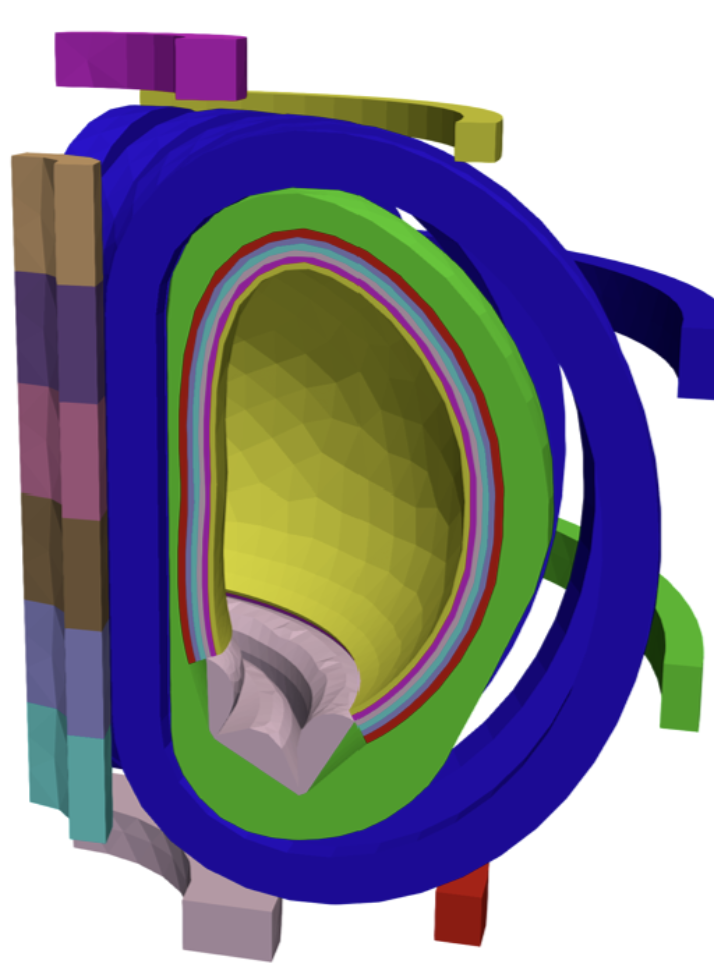
Figure 1: Tokamak model based on CAD generated with Paramak package.

We preview below the results of the coupled neutronics and heat transfer model from this workflow in Figure 3 and Figure 4 for the temperature distribution and tritium production rate density.

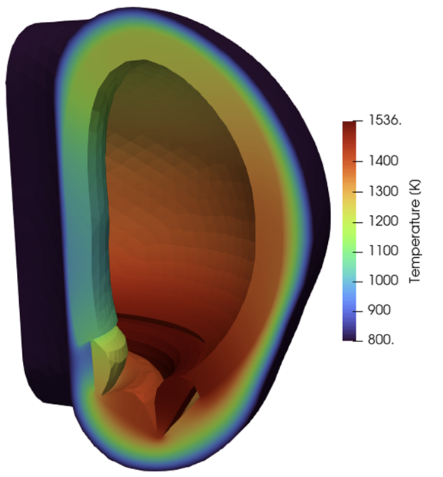
Figure 3: Example Paramak tokamak model temperature distribution result.

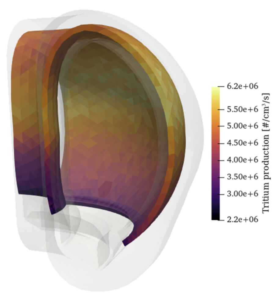
Figure 4: Example Paramak tokamak model tritium production rate density result.

This example demonstrates, on a simple mesh that can be made much more complex, how to:

Generate meshes for a coupled multiphysics SALAMANDER model.
Couple OpenMC (Romano et al., 2015) and SALAMANDER using Cardinal for fixed source Monte Carlo calculations.
Use Cardinal (Novak et al., 2022) to tally values of interest such as tritium production and heating which would be used in SALAMANDER to solve for the temperature and tritium distributions.

We describe this workflow for a generic CAD model which is extremely simplified for the purpose of the demonstration. Nonetheless, the same workflow is applicable to more complex CAD geometries. This model was also used in Eltawila et al. (2024) to perform mesh refinement studies to investigate how the mesh refinement level affects multiphysics results. The meshed geometry was prepared using direct accelerated geometry Monte Carlo (DAGMC) for particle transport, and a volumetric mesh was also prepared to be used in SALAMANDER’s finite element solver and to tally OpenMC results for heat source distribution and tritium production. Cardinal was used to run OpenMC Monte Carlo particle transport within SALAMANDER. The data transfer system transferred heat source and temperature distribution between OpenMC and SALAMANDER as shown in Figure 2, with coupling between neutron transport and heat conduction achieved via Picard iteration.

Figure 2: Illustration of OpenMC and MOOSE coupling.

Generating the meshes

The CAD model was first developed in Autodesk Fusion (This step can be done in any CAD generation software) and was imported into Coreform Cubit to assign blocks, materials, and side sets and generate the mesh (Figure 5). A corresponding DAGMC surface mesh (Figure 6) was exported directly from the meshed geometry in Cubit (by loading the volumetric meshed geometry in Cubit and exporting a DAGMC surface mesh).

In this example, tmesh_1.e (Figure 5) is the finite element mesh used in SALAMANDER on which the heat transfer physics is solved. tmesh_1.h5m (Figure 6) is the DAGMC surface mesh used for particle transport in OpenMC (which bounds the surfaces between different materials). Cardinal also allows for mesh tallying for tallying OpenMC results directly on the mesh overlayed on the OpenMC geometry which tmesh_1.e (Figure 5) could be used for as well as an unstructured volume mesh. This could be used by changing the tally type and adding a mesh template (tally_type = mesh, mesh_template = tmesh_1.e) in Cardinal Tally blocks.

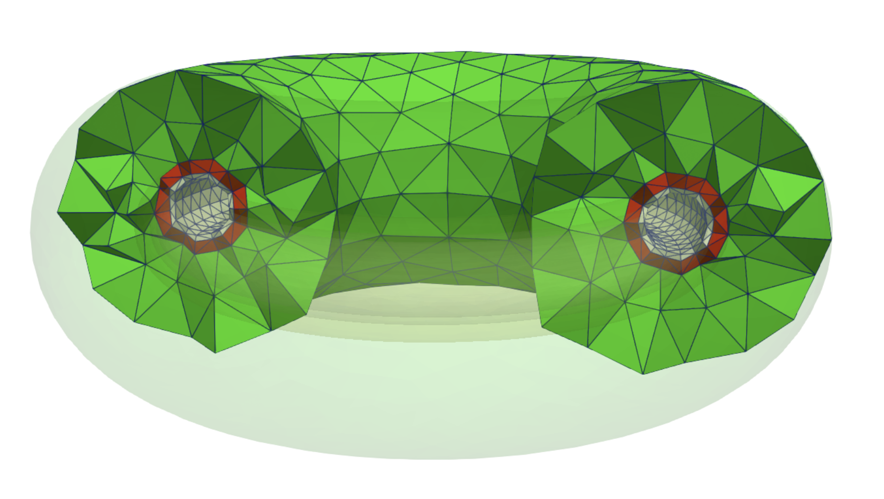
Figure 5: Model volumetric mesh.

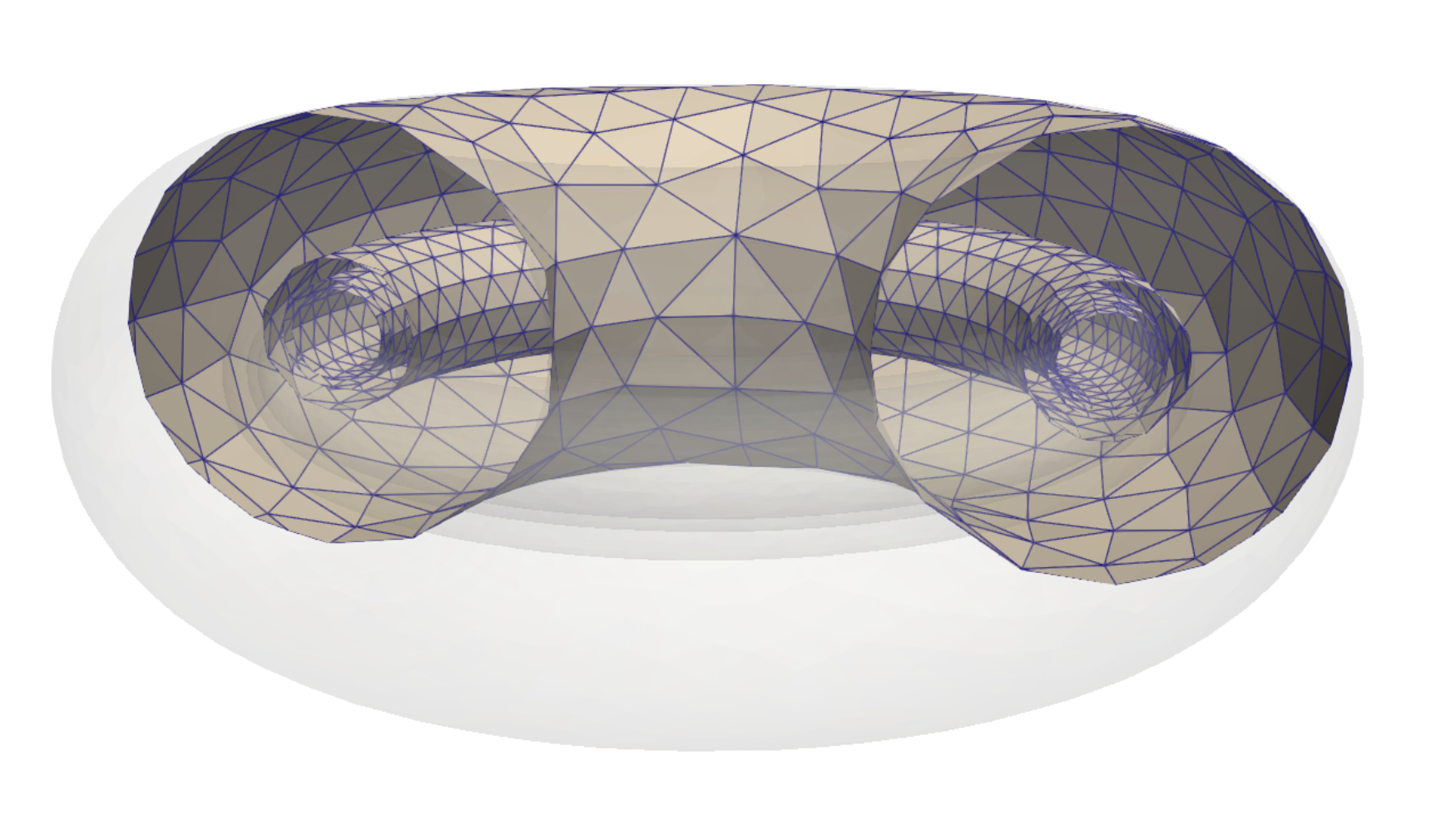
Figure 6: Model DAGMC mesh.

OpenMC

The OpenMC input files is as follows:

import openmc
import math

mat1 = openmc.Material(name="mat1")
mat1.set_density('g/cc', 19.30)
mat1.add_element('W', 1.0)

eurofer = openmc.Material(name="eurofer")
eurofer.add_element('Fe', 0.011   , 'wo')
eurofer.add_element('Al', 0.002   , 'wo')
eurofer.add_element('As', 0.0002  , 'wo')
eurofer.add_element('B', 0.0012  , 'wo')
eurofer.add_element('C', 0.0005  , 'wo')
eurofer.add_element('Co', 0.0005  , 'wo')
eurofer.add_element('Cr', 0.0005  , 'wo')
eurofer.add_element('Cu', 0.00005 , 'wo')
eurofer.add_element('Mn', 0.00005 , 'wo')
eurofer.add_element('Mo', 0.0001  , 'wo')
eurofer.add_element('N', 0.0001  , 'wo')
eurofer.add_element('Nb', 0.00005 , 'wo')
eurofer.add_element('Ni', 0.0003  , 'wo')
eurofer.add_element('O', 0.00005 , 'wo')
eurofer.add_element('P', 0.004   , 'wo')
eurofer.add_element('S', 0.0001  , 'wo')
eurofer.add_element('Sb', 0.09    , 'wo')
eurofer.add_element('Sn', 0.0001  , 'wo')
eurofer.add_element('Si', 0.0011  , 'wo')
eurofer.add_element('Ta', 0.00002 , 'wo')
eurofer.add_element('Ti', 0.0005  , 'wo')
eurofer.add_element('V', 0       , 'wo')
eurofer.add_element('W', 0.0001  , 'wo')
eurofer.add_element('Zr', 0.88698 , 'wo')
eurofer.set_density("g/cm3", 7.798)

Helium = openmc.Material(name="Helium")
Helium.add_element('He', 1.0)
Helium.set_density("kg/m3", 0.166)

mat2 = openmc.Material.mix_materials([eurofer, Helium], [0.65, 0.35], 'ao', name="mat2")

beryllium = openmc.Material(name="beryllium")
beryllium.add_element('Be', 1.0)
beryllium.set_density("g/cm3", 1.85)

Li4SiO4 = openmc.Material(name="Li4SiO4")
Li4SiO4.add_element('Li', 4.0)
Li4SiO4.add_element('Si', 1.0)
Li4SiO4.add_element('O', 4.0)
Li4SiO4.set_density("g/cm3", 2.39)

mat3 = openmc.Material.mix_materials([eurofer, beryllium, Li4SiO4, Helium], [0.1, 0.37, 0.15, 0.38], 'ao',name="mat3")

mats = openmc.Materials([mat1, eurofer, Helium,  mat2, beryllium, Li4SiO4,  mat3])
mats.export_to_xml()

pz = openmc.Plot()
pz.basis = 'yz'
pz.origin = (0.0, 0.0, 0.0)
pz.width = (200.0, 200.0)
pz.pixels = (500, 500)
pz.color_by = 'material'

px = openmc.Plot()
px.basis = 'xy'
px.origin = (0.0, 0.0, 0.0)
px.width = (200, 200)
px.pixels = (500, 500)
px.color_by = 'material'

plots = openmc.Plots([pz,px])
plots.export_to_xml()

settings = openmc.Settings()
settings.dagmc = True
settings.batches = 20
settings.particles = 10000000
settings.run_mode = "fixed source"

settings.temperature = {'default': 800.0,
                        'method': 'interpolation',
                        'range': (294.0, 3000.0),
                        'tolerance': 1000.0}

source = openmc.Source()

r = openmc.stats.PowerLaw(55, 65, 1.0)
phi = openmc.stats.Uniform(0.0, 2*math.pi)
z = openmc.stats.Discrete([0,], [1.0,])
spatial_dist = openmc.stats.CylindricalIndependent(r, phi, z)

source.angle = openmc.stats.Isotropic()
source.energy = openmc.stats.Discrete([14.08e6], [1.0])
source.space=spatial_dist
settings.source = source
settings.photon_transport = True
settings.export_to_xml()

dagmc_univ = openmc.DAGMCUniverse(filename='tmesh_1.h5m')

geometry = openmc.Geometry(root=dagmc_univ)
geometry.export_to_xml()

Cardinal

The Cardinal input files is shown below. The (MoabSkinner) was chosen in this model to update the DAGMC geometry from SALAMANDER mesh directly ensuring meshes matching which is further discussed in Eltawila et al. (2024) as well as the use of cell tallies.

# This test runs a coupled OpenMC and heat conduction model using a CAD-based geometry. The model
# uses an exodus (tmesh_1.e to use in MOOSE) and DAGMC (tmesh_1.h5m to use in OpenMC) meshes.
# openmc.i runs OpenMC to tally heating and tritium production taking cells temperature from MOOSE.

[Mesh<<<{"href": "../../syntax/Mesh/index.html"}>>>]
  [file]
    type = FileMeshGenerator<<<{"description": "Read a mesh from a file.", "href": "../../source/meshgenerators/FileMeshGenerator.html"}>>>
    file<<<{"description": "The filename to read."}>>> = tmesh_1.e
  []
  allow_renumbering = false
[]

[AuxVariables<<<{"href": "../../syntax/AuxVariables/index.html"}>>>]
  [cell_temperature]
    family<<<{"description": "Specifies the family of FE shape functions to use for this variable"}>>> = MONOMIAL
    order<<<{"description": "Specifies the order of the FE shape function to use for this variable (additional orders not listed are allowed)"}>>> = CONSTANT
  []
[]

[AuxKernels<<<{"href": "../../syntax/AuxKernels/index.html"}>>>]
  [cell_temperature]
    type = CellTemperatureAux<<<{"description": "OpenMC cell temperature (K), mapped to each MOOSE element", "href": "../../source/auxkernels/CellTemperatureAux.html"}>>>
    variable<<<{"description": "The name of the variable that this object applies to"}>>> = cell_temperature
  []
[]

[Problem<<<{"href": "../../syntax/Problem/index.html"}>>>]
  type = OpenMCCellAverageProblem
  cell_level = 0
  temperature_blocks = '1 2 3'
  temperature_variables = 'temperature'

  source_strength = 1e18 # Particles/s.
  volume_calculation = volume

  verbose = true
  particles = 500
  batches = 5

  skinner = moab
  [Tallies<<<{"href": "../../syntax/Problem/Tallies/index.html"}>>>]
    [heating_tritium]
      type = MeshTally<<<{"description": "A class which implements unstructured mesh tallies.", "href": "../../source/tallies/MeshTally.html"}>>>
      score<<<{"description": "Score(s) to use in the OpenMC tallies. If not specified, defaults to 'kappa_fission'"}>>> = 'heating_local H3_production'
      name<<<{"description": "Auxiliary variable name(s) to use for OpenMC tallies. If not specified, defaults to the names of the scores"}>>> = 'heating_local tritium_production'
      output<<<{"description": "UNRELAXED field(s) to output from OpenMC for each tally score. unrelaxed_tally_std_dev will write the standard deviation of each tally into auxiliary variables named *_std_dev. unrelaxed_tally_rel_error will write the relative standard deviation (unrelaxed_tally_std_dev / unrelaxed_tally) of each tally into auxiliary variables named *_rel_error. unrelaxed_tally will write the raw unrelaxed tally into auxiliary variables named *_raw (replace * with 'name')."}>>> = unrelaxed_tally_std_dev
    []
  []
[]

[UserObjects<<<{"href": "../../syntax/UserObjects/index.html"}>>>]
  [volume]
    type = OpenMCVolumeCalculation<<<{"description": "Stochastic volume calculation of the OpenMC cells which map to MOOSE", "href": "../../source/userobjects/OpenMCVolumeCalculation.html"}>>>
    n_samples<<<{"description": "Number of samples to use for the stochastic volume calculation"}>>> = 5000
  []
  [moab]
    type = MoabSkinner<<<{"description": "Re-generate the OpenMC geometry on-the-fly according to changes in the mesh geometry and/or contours in temperature and density", "href": "../../source/userobjects/MoabSkinner.html"}>>>
    temperature_min<<<{"description": "Lower bound of temperature bins"}>>> = 800
    temperature_max<<<{"description": "Upper bound of temperature bins"}>>> = 1500
    n_temperature_bins<<<{"description": "Number of temperature bins"}>>> = 10
    temperature<<<{"description": "Temperature variable by which to bin elements"}>>> = temperature
    build_graveyard<<<{"description": "Whether to build a graveyard around the geometry"}>>> = true
  []
[]

[Postprocessors<<<{"href": "../../syntax/Postprocessors/index.html"}>>>]
  [heat_source]
    type = ElementIntegralVariablePostprocessor<<<{"description": "Computes a volume integral of the specified variable", "href": "../../source/postprocessors/ElementIntegralVariablePostprocessor.html"}>>>
    variable<<<{"description": "The name of the variable that this object operates on"}>>> = heating_local
  []
  [tritium_production]
    type = ElementIntegralVariablePostprocessor<<<{"description": "Computes a volume integral of the specified variable", "href": "../../source/postprocessors/ElementIntegralVariablePostprocessor.html"}>>>
    variable<<<{"description": "The name of the variable that this object operates on"}>>> = tritium_production
  []
  [tritium_RelativeError]
    type = TallyRelativeError<<<{"description": "Maximum/minimum tally relative error", "href": "../../source/postprocessors/TallyRelativeError.html"}>>>
    tally_score<<<{"description": "Score to report the relative error. If there is just a single score, this defaults to that value"}>>> = H3_production
  []
  [heat_source_RelativeError]
    type = TallyRelativeError<<<{"description": "Maximum/minimum tally relative error", "href": "../../source/postprocessors/TallyRelativeError.html"}>>>
    tally_score<<<{"description": "Score to report the relative error. If there is just a single score, this defaults to that value"}>>> = heating_local
  []
[]

[Executioner<<<{"href": "../../syntax/Executioner/index.html"}>>>]
  type = Transient
[]

[Outputs<<<{"href": "../../syntax/Outputs/index.html"}>>>]
  exodus<<<{"description": "Output the results using the default settings for Exodus output."}>>> = true
  csv<<<{"description": "Output the scalar variable and postprocessors to a *.csv file using the default CSV output."}>>> = true
[]

SALAMANDER (MOOSE) Heat Transfer

The SALAMANDER input file is as follows:

# This test runs a coupled OpenMC and heat conduction model using a CAD-based geometry. The model
# uses an exodus (tmesh_1.e to use in MOOSE) and DAGMC (tmesh_1.h5m to use in OpenMC) meshes.
# solid.i solves heat conduction by taking heating results from OpenMC and sending back temperatures

# Conditions
initial_temperature = ${units 800.0 K}

# Material properties
thermal_conductivity_armor = ${units 1.64 W/m/K}
thermal_conductivity_FW = ${units 0.45 W/m/K}
thermal_conductivity_BM = ${units 0.65 W/m/K}

[Mesh<<<{"href": "../../syntax/Mesh/index.html"}>>>]
  [file]
    type = FileMeshGenerator<<<{"description": "Read a mesh from a file.", "href": "../../source/meshgenerators/FileMeshGenerator.html"}>>>
    file<<<{"description": "The filename to read."}>>> = tmesh_1.e
  []
[]

[Variables<<<{"href": "../../syntax/Variables/index.html"}>>>]
  [temperature]
    initial_condition<<<{"description": "Specifies a constant initial condition for this variable"}>>> = ${initial_temperature}
  []
[]

[AuxVariables<<<{"href": "../../syntax/AuxVariables/index.html"}>>>]
  [heat_source]
    family<<<{"description": "Specifies the family of FE shape functions to use for this variable"}>>> = MONOMIAL
    order<<<{"description": "Specifies the order of the FE shape function to use for this variable (additional orders not listed are allowed)"}>>> = CONSTANT
  []
[]

[Kernels<<<{"href": "../../syntax/Kernels/index.html"}>>>]
  [hc]
    type = HeatConduction<<<{"description": "Diffusive heat conduction term $-\\nabla\\cdot(k\\nabla T)$ of the thermal energy conservation equation", "href": "../../source/kernels/HeatConduction.html"}>>>
    variable<<<{"description": "The name of the variable that this residual object operates on"}>>> = temperature
  []
  [heat]
    type = CoupledForce<<<{"description": "Implements a source term proportional to the value of a coupled variable. Weak form: $(\\psi_i, -\\sigma v)$.", "href": "../../source/kernels/CoupledForce.html"}>>>
    variable<<<{"description": "The name of the variable that this residual object operates on"}>>> = temperature
    v<<<{"description": "The coupled variable which provides the force"}>>> = heat_source
  []
[]

[BCs<<<{"href": "../../syntax/BCs/index.html"}>>>]
  [surface]
    type = DirichletBC<<<{"description": "Imposes the essential boundary condition $u=g$, where $g$ is a constant, controllable value.", "href": "../../source/bcs/DirichletBC.html"}>>>
    variable<<<{"description": "The name of the variable that this residual object operates on"}>>> = temperature
    boundary<<<{"description": "The list of boundary IDs from the mesh where this object applies"}>>> = 1
    value<<<{"description": "Value of the BC"}>>> = ${initial_temperature}
  []
[]

[Materials<<<{"href": "../../syntax/Materials/index.html"}>>>]
  [k_1]
    type = GenericConstantMaterial<<<{"description": "Declares material properties based on names and values prescribed by input parameters.", "href": "../../source/materials/GenericConstantMaterial.html"}>>>
    prop_values<<<{"description": "The values associated with the named properties"}>>> = ${thermal_conductivity_armor}
    prop_names<<<{"description": "The names of the properties this material will have"}>>> = 'thermal_conductivity'
    block<<<{"description": "The list of blocks (ids or names) that this object will be applied"}>>> = 'Armour'
  []
  [k_2]
    type = GenericConstantMaterial<<<{"description": "Declares material properties based on names and values prescribed by input parameters.", "href": "../../source/materials/GenericConstantMaterial.html"}>>>
    prop_values<<<{"description": "The values associated with the named properties"}>>> = ${thermal_conductivity_FW}
    prop_names<<<{"description": "The names of the properties this material will have"}>>> = 'thermal_conductivity'
    block<<<{"description": "The list of blocks (ids or names) that this object will be applied"}>>> = 'FW'
  []
  [k_3]
    type = GenericConstantMaterial<<<{"description": "Declares material properties based on names and values prescribed by input parameters.", "href": "../../source/materials/GenericConstantMaterial.html"}>>>
    prop_values<<<{"description": "The values associated with the named properties"}>>> = ${thermal_conductivity_BM}
    prop_names<<<{"description": "The names of the properties this material will have"}>>> = 'thermal_conductivity'
    block<<<{"description": "The list of blocks (ids or names) that this object will be applied"}>>> = 'BM'
  []
[]

[Executioner<<<{"href": "../../syntax/Executioner/index.html"}>>>]
  type = Transient
  nl_abs_tol = 1e-8
  solve_type = 'NEWTON'
  num_steps = 2
[]

[Outputs<<<{"href": "../../syntax/Outputs/index.html"}>>>]
  exodus<<<{"description": "Output the results using the default settings for Exodus output."}>>> = true
  print_linear_residuals<<<{"description": "Enable printing of linear residuals to the screen (Console)"}>>> = false
  perf_graph<<<{"description": "Enable printing of the performance graph to the screen (Console)"}>>> = true
  csv<<<{"description": "Output the scalar variable and postprocessors to a *.csv file using the default CSV output."}>>> = true
[]

[MultiApps<<<{"href": "../../syntax/MultiApps/index.html"}>>>]
  [openmc]
    type = TransientMultiApp<<<{"description": "MultiApp for performing coupled simulations with the parent and sub-application both progressing in time.", "href": "../../source/multiapps/TransientMultiApp.html"}>>>
    app_type<<<{"description": "The type of application to build (applications not registered can be loaded with dynamic libraries. Parent application type will be used if not provided."}>>> = CardinalApp
    input_files<<<{"description": "The input file for each App.  If this parameter only contains one input file it will be used for all of the Apps.  When using 'positions_from_file' it is also admissable to provide one input_file per file."}>>> = 'openmc.i'
    execute_on<<<{"description": "The list of flag(s) indicating when this object should be executed. For a description of each flag, see https://mooseframework.inl.gov/source/interfaces/SetupInterface.html."}>>> = timestep_end
  []
[]

[Transfers<<<{"href": "../../syntax/Transfers/index.html"}>>>]
  [heat_source_from_openmc]
    type = MultiAppGeneralFieldShapeEvaluationTransfer<<<{"description": "Transfers field data at the MultiApp position using the finite element shape functions from the origin application.", "href": "../../source/transfers/MultiAppGeneralFieldShapeEvaluationTransfer.html"}>>>
    from_multi_app<<<{"description": "The name of the MultiApp to receive data from"}>>> = openmc
    variable<<<{"description": "The auxiliary variable to store the transferred values in."}>>> = heat_source
    source_variable<<<{"description": "The variable to transfer from."}>>> = heating_local
    from_postprocessors_to_be_preserved<<<{"description": "The name of the Postprocessor in the from-app to evaluate an adjusting factor."}>>> = heat_source
    to_postprocessors_to_be_preserved<<<{"description": "The name of the Postprocessor in the to-app to evaluate an adjusting factor."}>>> = source_integral
  []
  [temperature_to_openmc]
    type = MultiAppGeneralFieldShapeEvaluationTransfer<<<{"description": "Transfers field data at the MultiApp position using the finite element shape functions from the origin application.", "href": "../../source/transfers/MultiAppGeneralFieldShapeEvaluationTransfer.html"}>>>
    to_multi_app<<<{"description": "The name of the MultiApp to transfer the data to"}>>> = openmc
    variable<<<{"description": "The auxiliary variable to store the transferred values in."}>>> = temperature
    source_variable<<<{"description": "The variable to transfer from."}>>> = temperature
  []
[]

[Postprocessors<<<{"href": "../../syntax/Postprocessors/index.html"}>>>]
  [source_integral]
    type = ElementIntegralVariablePostprocessor<<<{"description": "Computes a volume integral of the specified variable", "href": "../../source/postprocessors/ElementIntegralVariablePostprocessor.html"}>>>
    variable<<<{"description": "The name of the variable that this object operates on"}>>> = heat_source
    execute_on<<<{"description": "The list of flag(s) indicating when this object should be executed. For a description of each flag, see https://mooseframework.inl.gov/source/interfaces/SetupInterface.html."}>>> = transfer
  []
  [max_temperature]
    type = NodalExtremeValue<<<{"description": "Finds either the min or max elemental value of a variable over the domain.", "href": "../../source/postprocessors/NodalExtremeValue.html"}>>>
    variable<<<{"description": "The name of the variable that this postprocessor operates on"}>>> = temperature
  []
[]

Execution

To generate OpenMC xml files, run:


python model.py

Then to run the coupled calculation:


mpiexec -np 2 salamander-opt -i solid.i --n-threads=2

This will run SALAMANDER with 2 MPI processes and 2 OpenMP threads per rank. To run the simulation faster, you can increase the parallel processes/threads, or simply decrease the number of particles used in OpenMC. When the simulation has completed, you will have created a number of different output files:

solid_out.e, an Exodus output with the solid mesh and solution from the MOOSE/SALAMANDER input file.
solid_out_openmc0.e, an Exodus output with the OpenMC solution and the data that was ultimately transferred in/out of OpenMC.

Results

The results of this simulation on the finest mesh are shown in Figure 7, Figure 8, and Table 1. More information, including a mesh sensitivity study, is available in Eltawila et al. (2024).

Temperature distribution result from [!cite](Eltawila2024PBNC).

Figure 7: Temperature distribution result from Eltawila et al. (2024).

Tritium production rate density result from [!cite](Eltawila2024PBNC).

Figure 8: Tritium production rate density result from Eltawila et al. (2024).

Table 1: Summary of the results from the coupled simulation published in Eltawila et al. (2024).

Parameter (Units)	Value	Units
Armor Max. Temperature	$var element = document.getElementById("moose-equation-2b7c5d8e-a247-4f02-9f4b-8d9a6e8066e9");katex.render("1062.4", element, {displayMode:false,throwOnError:false});$	`[K]`
First Wall Max. Temperature	$var element = document.getElementById("moose-equation-29985303-fa27-49df-89b6-abece350da25");katex.render("1057.6", element, {displayMode:false,throwOnError:false});$	`[K]`
Breeder Max. Temperature	$var element = document.getElementById("moose-equation-c569ae3d-02b3-4bc8-8436-507af4891706");katex.render("987.4", element, {displayMode:false,throwOnError:false});$	`[K]`
Heat Source	$var element = document.getElementById("moose-equation-4d96cba9-34b4-4ba5-8f9f-0101bde5f311");katex.render("2.44 \\times 10^5 \\pm 3 \\times 10^3", element, {displayMode:false,throwOnError:false});$	`[W]`
Tritium Production.	$var element = document.getElementById("moose-equation-e44e515a-a7a7-465c-ab3e-6796c48a60f7");katex.render("4.70 \\times 10^{13} \\pm 8 \\times 10^{11}", element, {displayMode:false,throwOnError:false});$	`[atoms/s]`

References

Mahmoud Eltawila, April J. Novak, Pierre-Clément A. Simon, Guillaume Giudicelli, and Derek Gaston. Investigation of cad-based geometry workflows for multiphysics fusion problems using openmc and moose. In Proceedings of the Pacific Basin Nuclear Conference (PBNC). Idaho Falls, ID, October 2024. American Nuclear Society. URL: https://www.ans.org/pubs/proceedings/article-56773/, doi:https://doi.org/10.13182/PBNC24-45030.

BibTeX

@inproceedings{Eltawila2024PBNC,
    author = "Eltawila, Mahmoud and Novak, April J. and Simon, Pierre-Clément A. and Giudicelli, Guillaume and Gaston, Derek",
    address = "Idaho Falls, ID",
    booktitle = "Proceedings of the Pacific Basin Nuclear Conference (PBNC)",
    month = "October",
    publisher = "American Nuclear Society",
    title = "Investigation of CAD-based Geometry Workflows for Multiphysics Fusion Problems Using OpenMC and MOOSE",
    year = "2024",
    page = "277-286",
    doi = "https://doi.org/10.13182/PBNC24-45030",
    url = "https://www.ans.org/pubs/proceedings/article-56773/"
}

RIS

TY  - CPAPER
AU  - Eltawila, Mahmoud
AU  - Novak, April J.
AU  - Simon, Pierre-Clément A.
AU  - Giudicelli, Guillaume
AU  - Gaston, Derek
TI  - Investigation of CAD-based Geometry Workflows for Multiphysics Fusion Problems Using OpenMC and MOOSE
T2  - Proceedings of the Pacific Basin Nuclear Conference (PBNC)
PY  - 2024
PB  - American Nuclear Society
CY  - Idaho Falls, ID
DO  - https://doi.org/10.13182/PBNC24-45030
UR  - https://www.ans.org/pubs/proceedings/article-56773/
ER  -

Plain Text

Mahmoud Eltawila, April J. Novak, Pierre-Clément A. Simon, Guillaume Giudicelli, and Derek Gaston. Investigation of cad-based geometry workflows for multiphysics fusion problems using openmc and moose. In Proceedings of the Pacific Basin Nuclear Conference (PBNC). Idaho Falls, ID, October 2024. American Nuclear Society. URL: https://www.ans.org/pubs/proceedings/article-56773/, doi:https://doi.org/10.13182/PBNC24-45030.

Guillaume Giudicelli, Alexander Lindsay, Logan Harbour, Casey Icenhour, Mengnan Li, Joshua E. Hansel, Peter German, Patrick Behne, Oana Marin, Roy H. Stogner, Jason M. Miller, Daniel Schwen, Yaqi Wang, Lynn Munday, Sebastian Schunert, Benjamin W. Spencer, Dewen Yushu, Antonio Recuero, Zachary M. Prince, Max Nezdyur, Tianchen Hu, Yinbin Miao, Yeon Sang Jung, Christopher Matthews, April Novak, Brandon Langley, Timothy Truster, Nuno Nobre, Brian Alger, David Andrš, Fande Kong, Robert Carlsen, Andrew E. Slaughter, John W. Peterson, Derek Gaston, and Cody Permann. 3.0 - MOOSE: enabling massively parallel multiphysics simulations. SoftwareX, 26:101690, 2024. URL: https://www.sciencedirect.com/science/article/pii/S235271102400061X, doi:https://doi.org/10.1016/j.softx.2024.101690.

BibTeX

@article{giudicelli2024moose,
    author = "Giudicelli, Guillaume and Lindsay, Alexander and Harbour, Logan and Icenhour, Casey and Li, Mengnan and Hansel, Joshua E. and German, Peter and Behne, Patrick and Marin, Oana and Stogner, Roy H. and Miller, Jason M. and Schwen, Daniel and Wang, Yaqi and Munday, Lynn and Schunert, Sebastian and Spencer, Benjamin W. and Yushu, Dewen and Recuero, Antonio and Prince, Zachary M. and Nezdyur, Max and Hu, Tianchen and Miao, Yinbin and Jung, Yeon Sang and Matthews, Christopher and Novak, April and Langley, Brandon and Truster, Timothy and Nobre, Nuno and Alger, Brian and Andr{\v{s}}, David and Kong, Fande and Carlsen, Robert and Slaughter, Andrew E. and Peterson, John W. and Gaston, Derek and Permann, Cody",
    title = "3.0 - {MOOSE}: Enabling massively parallel multiphysics simulations",
    year = "2024",
    journal = "{SoftwareX}",
    volume = "26",
    pages = "101690",
    issn = "2352-7110",
    doi = "https://doi.org/10.1016/j.softx.2024.101690",
    url = "https://www.sciencedirect.com/science/article/pii/S235271102400061X",
    keywords = "Framework, Finite-element, Finite-volume, Parallel, Multiphysics, Multiscale"
}

RIS

TY  - JOUR
AU  - Giudicelli, Guillaume
AU  - Lindsay, Alexander
AU  - Harbour, Logan
AU  - Icenhour, Casey
AU  - Li, Mengnan
AU  - Hansel, Joshua E.
AU  - German, Peter
AU  - Behne, Patrick
AU  - Marin, Oana
AU  - Stogner, Roy H.
AU  - Miller, Jason M.
AU  - Schwen, Daniel
AU  - Wang, Yaqi
AU  - Munday, Lynn
AU  - Schunert, Sebastian
AU  - Spencer, Benjamin W.
AU  - Yushu, Dewen
AU  - Recuero, Antonio
AU  - Prince, Zachary M.
AU  - Nezdyur, Max
AU  - Hu, Tianchen
AU  - Miao, Yinbin
AU  - Jung, Yeon Sang
AU  - Matthews, Christopher
AU  - Novak, April
AU  - Langley, Brandon
AU  - Truster, Timothy
AU  - Nobre, Nuno
AU  - Alger, Brian
AU  - Andrš, David
AU  - Kong, Fande
AU  - Carlsen, Robert
AU  - Slaughter, Andrew E.
AU  - Peterson, John W.
AU  - Gaston, Derek
AU  - Permann, Cody
TI  - 3.0 - MOOSE: Enabling massively parallel multiphysics simulations
JO  - SoftwareX
PY  - 2024
VL  - 26
DO  - https://doi.org/10.1016/j.softx.2024.101690
UR  - https://www.sciencedirect.com/science/article/pii/S235271102400061X
SP  - 101690
ER  -

Plain Text

Guillaume Giudicelli, Alexander Lindsay, Logan Harbour, Casey Icenhour, Mengnan Li, Joshua E. Hansel, Peter German, Patrick Behne, Oana Marin, Roy H. Stogner, Jason M. Miller, Daniel Schwen, Yaqi Wang, Lynn Munday, Sebastian Schunert, Benjamin W. Spencer, Dewen Yushu, Antonio Recuero, Zachary M. Prince, Max Nezdyur, Tianchen Hu, Yinbin Miao, Yeon Sang Jung, Christopher Matthews, April Novak, Brandon Langley, Timothy Truster, Nuno Nobre, Brian Alger, David Andrš, Fande Kong, Robert Carlsen, Andrew E. Slaughter, John W. Peterson, Derek Gaston, and Cody Permann. 3.0 - MOOSE: enabling massively parallel multiphysics simulations. SoftwareX, 26:101690, 2024. URL: https://www.sciencedirect.com/science/article/pii/S235271102400061X, doi:https://doi.org/10.1016/j.softx.2024.101690.

A.J. Novak, D. Andrs, P. Shriwise, J. Fang, H. Yuan, D. Shaver, E. Merzari, P.K. Romano, and R.C. Martineau. Coupled Monte Carlo and Thermal-Fluid Modeling of High Temperature Gas Reactors Using Cardinal. Annals of Nuclear Energy, 177:109310, 2022. doi:10.1016/j.anucene.2022.109310.

BibTeX

@Article{novak2022_cardinal,
    author = "Novak, A.J. and Andrs, D. and Shriwise, P. and Fang, J. and Yuan, H. and Shaver, D. and Merzari, E. and Romano, P.K. and Martineau, R.C.",
    title = "{Coupled {Monte} {Carlo} and Thermal-Fluid Modeling of High Temperature Gas Reactors Using {Cardinal}}",
    journal = "Annals of Nuclear Energy",
    year = "2022",
    volume = "177",
    pages = "109310",
    DOI = "10.1016/j.anucene.2022.109310"
}

RIS

TY  - JOUR
AU  - Novak, A.J.
AU  - Andrs, D.
AU  - Shriwise, P.
AU  - Fang, J.
AU  - Yuan, H.
AU  - Shaver, D.
AU  - Merzari, E.
AU  - Romano, P.K.
AU  - Martineau, R.C.
TI  - Coupled Monte Carlo and Thermal-Fluid Modeling of High Temperature Gas Reactors Using Cardinal
JO  - Annals of Nuclear Energy
PY  - 2022
VL  - 177
DO  - 10.1016/j.anucene.2022.109310
SP  - 109310
ER  -

Plain Text

A.J. Novak, D. Andrs, P. Shriwise, J. Fang, H. Yuan, D. Shaver, E. Merzari, P.K. Romano, and R.C. Martineau. Coupled Monte Carlo and Thermal-Fluid Modeling of High Temperature Gas Reactors Using Cardinal. Annals of Nuclear Energy, 177:109310, 2022. doi:10.1016/j.anucene.2022.109310.

P.K. Romano, N.E. Horelik, B.R. Herman, A.G. Nelson, B. Forget, and K. Smith. OpenMC: A State-of-the-Art Monte Carlo Code for Research and Development. Annals of Nuclear Energy, 82:90–97, 2015. doi:10.1016/j.anucene.2014.07.048.

BibTeX

@Article{openmc,
    author = "Romano, P.K. and Horelik, N.E. and Herman, B.R. and Nelson, A.G. and Forget, B. and Smith, K.",
    title = "{OpenMC: A State-of-the-Art {Monte} {Carlo} Code for Research and Development}",
    journal = "Annals of Nuclear Energy",
    year = "2015",
    volume = "82",
    pages = "90--97",
    DOI = "10.1016/j.anucene.2014.07.048"
}

RIS

TY  - JOUR
AU  - Romano, P.K.
AU  - Horelik, N.E.
AU  - Herman, B.R.
AU  - Nelson, A.G.
AU  - Forget, B.
AU  - Smith, K.
TI  - OpenMC: A State-of-the-Art Monte Carlo Code for Research and Development
JO  - Annals of Nuclear Energy
PY  - 2015
VL  - 82
DO  - 10.1016/j.anucene.2014.07.048
SP  - 90
EP  - 97
ER  -

Plain Text

P.K. Romano, N.E. Horelik, B.R. Herman, A.G. Nelson, B. Forget, and K. Smith. OpenMC: A State-of-the-Art Monte Carlo Code for Research and Development. Annals of Nuclear Energy, 82:90–97, 2015. doi:10.1016/j.anucene.2014.07.048.

Jonathan Shimwell, John Billingsley, Rémi Delaporte-Mathurin, Declan Morbey, Matthew Bluteau, Patrick Shriwise, and Andrew Davis. The paramak: automated parametric geometry construction for fusion reactor designs. F1000Research, 2021.

BibTeX

@article{shimwell2021paramak,
    author = "Shimwell, Jonathan and Billingsley, John and Delaporte-Mathurin, R{\'e}mi and Morbey, Declan and Bluteau, Matthew and Shriwise, Patrick and Davis, Andrew",
    title = "The Paramak: automated parametric geometry construction for fusion reactor designs.",
    journal = "F1000Research",
    volume = "10",
    year = "2021",
    publisher = "Faculty of 1000 Ltd"
}

RIS

TY  - JOUR
AU  - Shimwell, Jonathan
AU  - Billingsley, John
AU  - Delaporte-Mathurin, Rémi
AU  - Morbey, Declan
AU  - Bluteau, Matthew
AU  - Shriwise, Patrick
AU  - Davis, Andrew
TI  - The Paramak: automated parametric geometry construction for fusion reactor designs.
JO  - F1000Research
PY  - 2021
VL  - 10
PB  - Faculty of 1000 Ltd
ER  -

Plain Text

Jonathan Shimwell, John Billingsley, Rémi Delaporte-Mathurin, Declan Morbey, Matthew Bluteau, Patrick Shriwise, and Andrew Davis. The paramak: automated parametric geometry construction for fusion reactor designs. F1000Research, 2021.

(test/tests/neutronics/cad_workflow/model.py)

import openmc
import math

mat1 = openmc.Material(name="mat1")
mat1.set_density('g/cc', 19.30)
mat1.add_element('W', 1.0)

eurofer = openmc.Material(name="eurofer")
eurofer.add_element('Fe', 0.011   , 'wo')
eurofer.add_element('Al', 0.002   , 'wo')
eurofer.add_element('As', 0.0002  , 'wo')
eurofer.add_element('B', 0.0012  , 'wo')
eurofer.add_element('C', 0.0005  , 'wo')
eurofer.add_element('Co', 0.0005  , 'wo')
eurofer.add_element('Cr', 0.0005  , 'wo')
eurofer.add_element('Cu', 0.00005 , 'wo')
eurofer.add_element('Mn', 0.00005 , 'wo')
eurofer.add_element('Mo', 0.0001  , 'wo')
eurofer.add_element('N', 0.0001  , 'wo')
eurofer.add_element('Nb', 0.00005 , 'wo')
eurofer.add_element('Ni', 0.0003  , 'wo')
eurofer.add_element('O', 0.00005 , 'wo')
eurofer.add_element('P', 0.004   , 'wo')
eurofer.add_element('S', 0.0001  , 'wo')
eurofer.add_element('Sb', 0.09    , 'wo')
eurofer.add_element('Sn', 0.0001  , 'wo')
eurofer.add_element('Si', 0.0011  , 'wo')
eurofer.add_element('Ta', 0.00002 , 'wo')
eurofer.add_element('Ti', 0.0005  , 'wo')
eurofer.add_element('V', 0       , 'wo')
eurofer.add_element('W', 0.0001  , 'wo')
eurofer.add_element('Zr', 0.88698 , 'wo')
eurofer.set_density("g/cm3", 7.798)

Helium = openmc.Material(name="Helium")
Helium.add_element('He', 1.0)
Helium.set_density("kg/m3", 0.166)

mat2 = openmc.Material.mix_materials([eurofer, Helium], [0.65, 0.35], 'ao', name="mat2")

beryllium = openmc.Material(name="beryllium")
beryllium.add_element('Be', 1.0)
beryllium.set_density("g/cm3", 1.85)

Li4SiO4 = openmc.Material(name="Li4SiO4")
Li4SiO4.add_element('Li', 4.0)
Li4SiO4.add_element('Si', 1.0)
Li4SiO4.add_element('O', 4.0)
Li4SiO4.set_density("g/cm3", 2.39)

mat3 = openmc.Material.mix_materials([eurofer, beryllium, Li4SiO4, Helium], [0.1, 0.37, 0.15, 0.38], 'ao',name="mat3")

mats = openmc.Materials([mat1, eurofer, Helium,  mat2, beryllium, Li4SiO4,  mat3])
mats.export_to_xml()

pz = openmc.Plot()
pz.basis = 'yz'
pz.origin = (0.0, 0.0, 0.0)
pz.width = (200.0, 200.0)
pz.pixels = (500, 500)
pz.color_by = 'material'

px = openmc.Plot()
px.basis = 'xy'
px.origin = (0.0, 0.0, 0.0)
px.width = (200, 200)
px.pixels = (500, 500)
px.color_by = 'material'

plots = openmc.Plots([pz,px])
plots.export_to_xml()

settings = openmc.Settings()
settings.dagmc = True
settings.batches = 20
settings.particles = 10000000
settings.run_mode = "fixed source"

settings.temperature = {'default': 800.0,
                        'method': 'interpolation',
                        'range': (294.0, 3000.0),
                        'tolerance': 1000.0}

source = openmc.Source()

r = openmc.stats.PowerLaw(55, 65, 1.0)
phi = openmc.stats.Uniform(0.0, 2*math.pi)
z = openmc.stats.Discrete([0,], [1.0,])
spatial_dist = openmc.stats.CylindricalIndependent(r, phi, z)

source.angle = openmc.stats.Isotropic()
source.energy = openmc.stats.Discrete([14.08e6], [1.0])
source.space=spatial_dist
settings.source = source
settings.photon_transport = True
settings.export_to_xml()

dagmc_univ = openmc.DAGMCUniverse(filename='tmesh_1.h5m')

geometry = openmc.Geometry(root=dagmc_univ)
geometry.export_to_xml()

(test/tests/neutronics/cad_workflow/openmc.i)

# This test runs a coupled OpenMC and heat conduction model using a CAD-based geometry. The model
# uses an exodus (tmesh_1.e to use in MOOSE) and DAGMC (tmesh_1.h5m to use in OpenMC) meshes.
# openmc.i runs OpenMC to tally heating and tritium production taking cells temperature from MOOSE.

[Mesh]
  [file]
    type = FileMeshGenerator
    file = tmesh_1.e
  []
  allow_renumbering = false
[]

[AuxVariables]
  [cell_temperature]
    family = MONOMIAL
    order = CONSTANT
  []
[]

[AuxKernels]
  [cell_temperature]
    type = CellTemperatureAux
    variable = cell_temperature
  []
[]

[Problem]
  type = OpenMCCellAverageProblem
  cell_level = 0
  temperature_blocks = '1 2 3'
  temperature_variables = 'temperature'

  source_strength = 1e18 # Particles/s.
  volume_calculation = volume

  verbose = true
  particles = 500
  batches = 5

  skinner = moab
  [Tallies]
    [heating_tritium]
      type = MeshTally
      score = 'heating_local H3_production'
      name = 'heating_local tritium_production'
      output = unrelaxed_tally_std_dev
    []
  []
[]

[UserObjects]
  [volume]
    type = OpenMCVolumeCalculation
    n_samples = 5000
  []
  [moab]
    type = MoabSkinner
    temperature_min = 800
    temperature_max = 1500
    n_temperature_bins = 10
    temperature = temperature
    build_graveyard = true
  []
[]

[Postprocessors]
  [heat_source]
    type = ElementIntegralVariablePostprocessor
    variable = heating_local
  []
  [tritium_production]
    type = ElementIntegralVariablePostprocessor
    variable = tritium_production
  []
  [tritium_RelativeError]
    type = TallyRelativeError
    tally_score = H3_production
  []
  [heat_source_RelativeError]
    type = TallyRelativeError
    tally_score = heating_local
  []
[]

[Executioner]
  type = Transient
[]

[Outputs]
  exodus = true
  csv = true
[]

(test/tests/neutronics/cad_workflow/solid.i)

# This test runs a coupled OpenMC and heat conduction model using a CAD-based geometry. The model
# uses an exodus (tmesh_1.e to use in MOOSE) and DAGMC (tmesh_1.h5m to use in OpenMC) meshes.
# solid.i solves heat conduction by taking heating results from OpenMC and sending back temperatures

# Conditions
initial_temperature = ${units 800.0 K}

# Material properties
thermal_conductivity_armor = ${units 1.64 W/m/K}
thermal_conductivity_FW = ${units 0.45 W/m/K}
thermal_conductivity_BM = ${units 0.65 W/m/K}

[Mesh]
  [file]
    type = FileMeshGenerator
    file = tmesh_1.e
  []
[]

[Variables]
  [temperature]
    initial_condition = ${initial_temperature}
  []
[]

[AuxVariables]
  [heat_source]
    family = MONOMIAL
    order = CONSTANT
  []
[]

[Kernels]
  [hc]
    type = HeatConduction
    variable = temperature
  []
  [heat]
    type = CoupledForce
    variable = temperature
    v = heat_source
  []
[]

[BCs]
  [surface]
    type = DirichletBC
    variable = temperature
    boundary = 1
    value = ${initial_temperature}
  []
[]

[Materials]
  [k_1]
    type = GenericConstantMaterial
    prop_values = ${thermal_conductivity_armor}
    prop_names = 'thermal_conductivity'
    block = 'Armour'
  []
  [k_2]
    type = GenericConstantMaterial
    prop_values = ${thermal_conductivity_FW}
    prop_names = 'thermal_conductivity'
    block = 'FW'
  []
  [k_3]
    type = GenericConstantMaterial
    prop_values = ${thermal_conductivity_BM}
    prop_names = 'thermal_conductivity'
    block = 'BM'
  []
[]

[Executioner]
  type = Transient
  nl_abs_tol = 1e-8
  solve_type = 'NEWTON'
  num_steps = 2
[]

[Outputs]
  exodus = true
  print_linear_residuals = false
  perf_graph = true
  csv = true
[]

[MultiApps]
  [openmc]
    type = TransientMultiApp
    app_type = CardinalApp
    input_files = 'openmc.i'
    execute_on = timestep_end
  []
[]

[Transfers]
  [heat_source_from_openmc]
    type = MultiAppGeneralFieldShapeEvaluationTransfer
    from_multi_app = openmc
    variable = heat_source
    source_variable = heating_local
    from_postprocessors_to_be_preserved = heat_source
    to_postprocessors_to_be_preserved = source_integral
  []
  [temperature_to_openmc]
    type = MultiAppGeneralFieldShapeEvaluationTransfer
    to_multi_app = openmc
    variable = temperature
    source_variable = temperature
  []
[]

[Postprocessors]
  [source_integral]
    type = ElementIntegralVariablePostprocessor
    variable = heat_source
    execute_on = transfer
  []
  [max_temperature]
    type = NodalExtremeValue
    variable = temperature
  []
[]

Generating the meshes
OpenMC
Cardinal
SALAMANDER ( MOOSE ) Heat Transfer
Execution
Results
References