(tmap8/test/tests/val-2g/val-2g_trapping.i)
# Validation Problem #2g for TMAP8
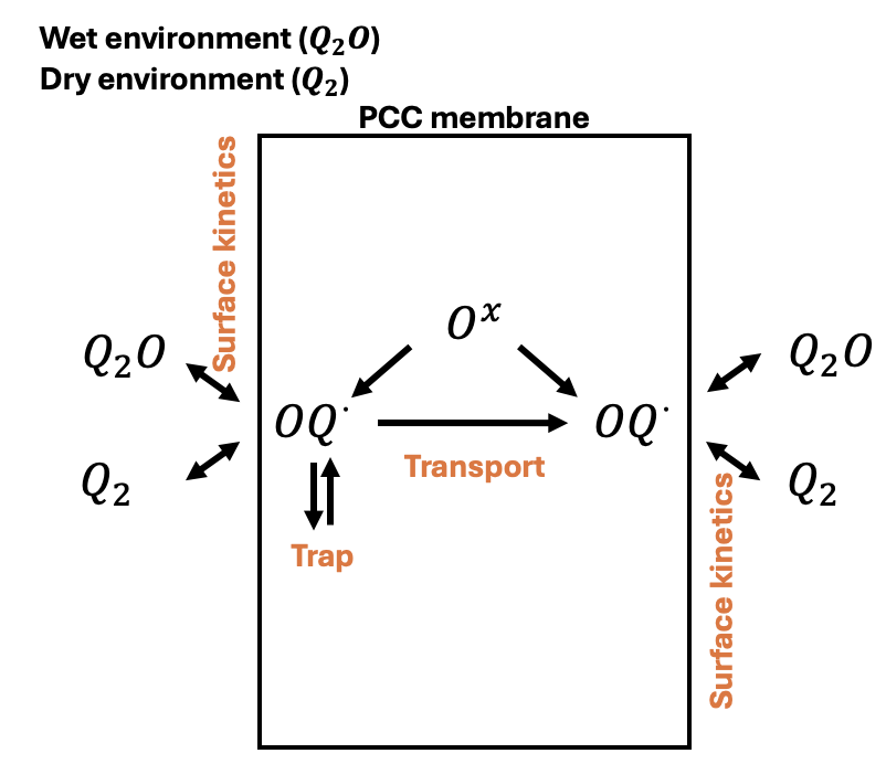
# Deuterium Transport in Proton-Conducting Ceramics
# Diffusion, Trapping, Surface Reaction under Wet and Dry Considered, No Soret effect
# Physical constants
R = '${units 8.31446261815324 J/mol/K}' # ideal gas constant based on number used in include/utils/PhysicalConstants.h
eV_to_J = '${units 1.602176634e-19 eV/J}' # eV to J conversion factor based on number used in include/utils/PhysicalConstants.h
N_a = '${units 6.02214076e23 at/mol}' # Avogadro's number based on number used in include/utils/PhysicalConstants.h
k_B = '${units 8.61733e-5 eV/K}' # Boltzmann constant in eV
# thermal parameters
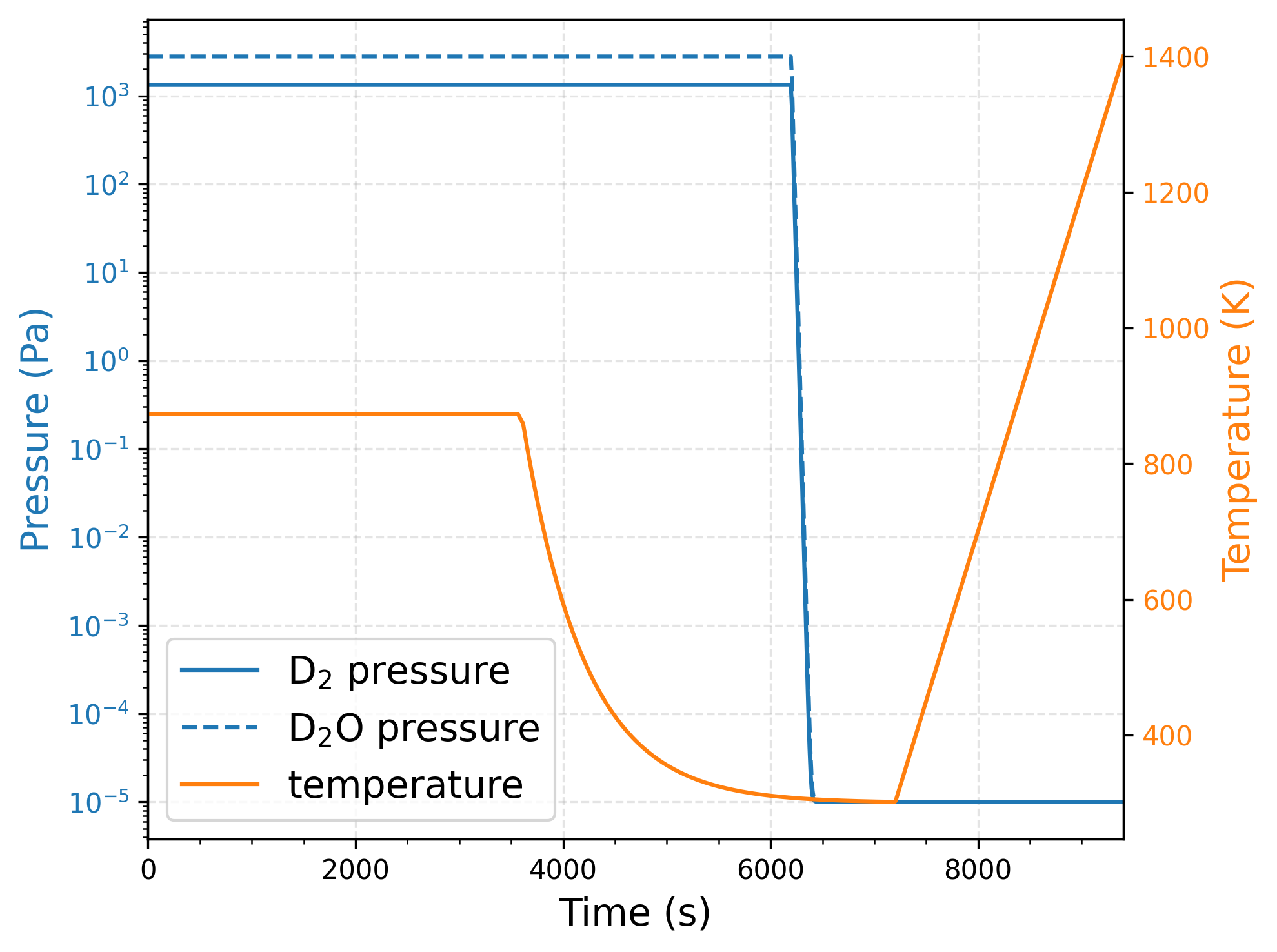
temperature_low = '${units 300 K}'
temperature_initial = '${units 873 K}'
temperature_high = '${units 1400 K}'
temperature_rate = '${units 0.5 K/s}'
# Model parameters
dissolve_duration = '${units 1 h -> s}'
cooldown_time_constant = '${units ${fparse 10*60} s}'
cooldown_duration = '${units 1 h -> s}'
desorption_duration = '${fparse (temperature_high - temperature_low) / temperature_rate}'
endtime = '${units ${fparse dissolve_duration + cooldown_duration + desorption_duration} s}'
dt_start_charging = '${units 1e-4 s}'
bound_value_min = '${units -1e-20 at/mum^3}'
# Geometry and mesh
length = '${units 0.5 mm -> mum}'
edge_number = 200
boundary_mesh = '${units 12 mum}'
num_nodes = 600
Area = '${units ${fparse 7.7e-3 * 2.2e-3} m^2 -> mum^2}'
# Material properties
density_BZY20 = '${units 5.98 g/cm^3 -> g/m^3}'
molar_mass_BZY20 = '${units 276.085 g/mol}'
N = '${units ${fparse density_BZY20 / molar_mass_BZY20 * N_a} at/m^3 -> at/mum^3}' # 1.3043649601e10
# Initial concentrations
OT_concentration_initial = 0
hydration_limit_S = 0.1
oxygen_vacancy_concentration_initial = '${units ${fparse hydration_limit_S / 2 * N} at/mum^3}'
oxygen_concentration_initial = '${units ${fparse 3 * N - oxygen_vacancy_concentration_initial - OT_concentration_initial} at/mum^3}'
electron_concentration_initial = '${units ${fparse 10 ^ electron_concentration_initial_expo * N} at/mum^3}' # 0.001
# Traps parameters
initial_concentration_trap_1 = 0 # (-)
detrapping_energy_1 = '${fparse detrapping_energy_1_ev / k_B}'
trapping_site_fraction_1 = ${fparse 3 * 10 ^ trapping_site_fraction_1_expo} # (-)
trapping_rate_prefactor = '${units ${fparse 4.8 * 10 ^ trapping_rate_prefactor_expo} 1/s}' # 9.1316e12
release_rate_profactor = '${units ${fparse 2.6 * 10 ^ release_rate_profactor_expo }1/s}' # 8.4e12
trapping_energy = '${fparse trapping_energy_ev / k_B}'
trap_per_free_1 = 1e0 # (-)
##### Dry Pressure conditions
pressure_T2_high = '${units 1.33e3 Pa}'
pressure_T2_low = '${units 1e-5 Pa}'
pressure_T2O_dry = '${units 0 Pa}' # We assume the pressure of T2O is 0
##### Wet Pressure conditions
pressure_T2O_high = '${units 2.8e3 Pa}'
pressure_T2O_low = '${units 1e-5 Pa}'
pressure_T2_wet = '${units 0 Pa}' # We assume the pressure of T2 is 0
# chemical_reaction
T2O_reaction_forward_value = '${units ${fparse 2 * 10 ^ T2O_reaction_forward_value_expo} m^4/at/s -> mum^4/at/s}'
T2_reaction_forward_value = '${units ${fparse 2 * 10 ^ T2_reaction_forward_value_expo} m^4/at/s -> mum^4/at/s}'
# Materials diffusivities (Deuterium: diffusivity and solubility data from Hossain 2020)
diffusivity_OT_prefactor = '${units ${fparse diffusivity_OT_prefactor_m2s * sqrt(3/2)} m^2/s -> mum^2/s}'
diffusivity_OT_energy = '${units ${fparse diffusivity_OT_energy_ev * eV_to_J * N_a} J/mol}'
diffusivity_V_O_prefactor = '${units ${diffusivity_V_O_prefactor_m2s} m^2/s -> mum^2/s}'
diffusivity_e_prefactor = '${units ${diffusivity_e_prefactor_m2s} m^2/s -> mum^2/s}'
[Mesh]
active = 'cmg_edge'
[cmg_edge]
type = CartesianMeshGenerator
dim = 1
dx = '${boundary_mesh} ${fparse length - 2 * boundary_mesh} ${boundary_mesh}'
ix = '${edge_number} ${fparse num_nodes - 2*edge_number} ${edge_number}'
subdomain_id = '0 0 0'
[]
[cmg]
type = CartesianMeshGenerator
dim = 1
dx = '${fparse length}'
ix = '${fparse num_nodes}'
subdomain_id = '0'
[]
[]
[Variables]
#### Dry variable
[OT_concentration_dry] # (atoms/microns^3)
initial_condition = ${OT_concentration_initial}
[]
[Oxygen_vacancy_concentration_dry]
initial_condition = ${oxygen_vacancy_concentration_initial}
[]
[electron_concentration_dry]
initial_condition = ${electron_concentration_initial}
[]
[trapped_1_dry]
order = FIRST
family = LAGRANGE
initial_condition = '${fparse initial_concentration_trap_1 * trapping_site_fraction_1 * N}'
[]
#### Wet variable
[OT_concentration_wet] # (atoms/microns^3)
initial_condition = ${OT_concentration_initial}
[]
[Oxygen_vacancy_concentration_wet]
initial_condition = ${oxygen_vacancy_concentration_initial}
[]
[electron_concentration_wet]
initial_condition = ${electron_concentration_initial}
[]
[trapped_1_wet]
order = FIRST
family = LAGRANGE
initial_condition = '${fparse initial_concentration_trap_1 * trapping_site_fraction_1 * N}'
[]
[]
[Bounds]
[concentration_dry_lower_bound]
type = ConstantBounds
variable = bounds_dummy
bounded_variable = OT_concentration_dry
bound_type = lower
bound_value = ${bound_value_min}
[]
[trap1_dry_lower_bound]
type = ConstantBounds
variable = bounds_dummy
bounded_variable = trapped_1_dry
bound_type = lower
bound_value = ${bound_value_min}
[]
[concentration_wet_lower_bound]
type = ConstantBounds
variable = bounds_dummy
bounded_variable = OT_concentration_wet
bound_type = lower
bound_value = ${bound_value_min}
[]
[trap1_wet_lower_bound]
type = ConstantBounds
variable = bounds_dummy
bounded_variable = trapped_1_wet
bound_type = lower
bound_value = ${bound_value_min}
[]
[]
[AuxVariables]
[bounds_dummy]
order = FIRST
family = LAGRANGE
[]
[temperature]
initial_condition = ${temperature_initial}
[]
#### Dry auxvariable
[pressure_T2_dry]
initial_condition = ${pressure_T2_high}
[]
[Oxygen_concentration_dry]
initial_condition = ${oxygen_concentration_initial}
[]
#### Wet auxvariable
[pressure_T2O_wet]
initial_condition = ${pressure_T2O_high}
[]
[Oxygen_concentration_wet]
initial_condition = ${oxygen_concentration_initial}
[]
[]
[AuxKernels]
[temperature_Aux]
type = FunctionAux
variable = temperature
function = Temperature_function
[]
#### Dry auxkernels
[pressure_T2_dry_Aux]
type = FunctionAux
variable = pressure_T2_dry
function = Pressure_T2_dry_function
[]
[Oxygen_concentration_dry_Aux] # at/mum^3
type = ParsedAux
variable = Oxygen_concentration_dry
coupled_variables = 'Oxygen_vacancy_concentration_dry OT_concentration_dry'
expression = '3 * ${N} - Oxygen_vacancy_concentration_dry - OT_concentration_dry'
[]
#### Wet auxkernels
[pressure_T2O_wet_Aux]
type = FunctionAux
variable = pressure_T2O_wet
function = Pressure_T2O_wet_function
[]
[Oxygen_concentration_wet_Aux] # at/mum^3
type = ParsedAux
variable = Oxygen_concentration_wet
coupled_variables = 'Oxygen_vacancy_concentration_wet OT_concentration_wet'
expression = '3 * ${N} - Oxygen_vacancy_concentration_wet - OT_concentration_wet'
[]
[]
[Problem]
type = ReferenceResidualProblem
extra_tag_vectors = 'ref'
reference_vector = 'ref'
[]
[Kernels]
#### Dry kernels
[time_OT_dry]
type = ADTimeDerivative
variable = OT_concentration_dry
extra_vector_tags = ref
[]
[diffusion_OT_dry]
type = ADMatDiffusion
variable = OT_concentration_dry
diffusivity = diffusivity_OT
extra_vector_tags = ref
[]
[time_V_O_dry]
type = ADTimeDerivative
variable = Oxygen_vacancy_concentration_dry
extra_vector_tags = ref
[]
[diffusion_V_O_dry]
type = ADMatDiffusion
variable = Oxygen_vacancy_concentration_dry
diffusivity = diffusivity_V_O
extra_vector_tags = ref
[]
[time_e_dry]
type = ADTimeDerivative
variable = electron_concentration_dry
extra_vector_tags = ref
[]
[diffusion_e_dry]
type = ADMatDiffusion
variable = electron_concentration_dry
diffusivity = diffusivity_e
extra_vector_tags = ref
[]
# trapping kernel
[coupled_time_trap_1_dry]
type = ADCoefCoupledTimeDerivative
variable = OT_concentration_dry
v = trapped_1_dry
coef = ${trap_per_free_1}
block = 0
extra_vector_tags = ref
[]
#### Wet kernels
[time_OT_wet]
type = ADTimeDerivative
variable = OT_concentration_wet
extra_vector_tags = ref
[]
[diffusion_OT_wet]
type = ADMatDiffusion
variable = OT_concentration_wet
diffusivity = diffusivity_OT
extra_vector_tags = ref
[]
[time_V_O_wet]
type = ADTimeDerivative
variable = Oxygen_vacancy_concentration_wet
extra_vector_tags = ref
[]
[diffusion_V_O_wet]
type = ADMatDiffusion
variable = Oxygen_vacancy_concentration_wet
diffusivity = diffusivity_V_O
extra_vector_tags = ref
[]
[time_e_wet]
type = ADTimeDerivative
variable = electron_concentration_wet
extra_vector_tags = ref
[]
[diffusion_e_wet]
type = ADMatDiffusion
variable = electron_concentration_wet
diffusivity = diffusivity_e
extra_vector_tags = ref
[]
# trapping kernel
[coupled_time_trap_1_wet]
type = ADCoefCoupledTimeDerivative
variable = OT_concentration_wet
v = trapped_1_wet
coef = ${trap_per_free_1}
block = 0
extra_vector_tags = ref
[]
[]
[NodalKernels]
#### First traps under dry
[time_1_dry]
type = TimeDerivativeNodalKernel
variable = trapped_1_dry
[]
[trapping_1_dry]
type = TrappingNodalKernel
variable = trapped_1_dry
mobile_concentration = OT_concentration_dry
alpha_t = '${trapping_rate_prefactor}'
trapping_energy = '${trapping_energy}'
N = '${N}'
Ct0 = '${trapping_site_fraction_1}'
temperature = 'temperature'
trap_per_free = '${trap_per_free_1}'
extra_vector_tags = ref
[]
[release_1_dry]
type = ReleasingNodalKernel
variable = trapped_1_dry
alpha_r = '${release_rate_profactor}'
detrapping_energy = '${detrapping_energy_1}'
temperature = 'temperature'
[]
#### First traps under wet
[time_1_wet]
type = TimeDerivativeNodalKernel
variable = trapped_1_wet
[]
[trapping_1_wet]
type = TrappingNodalKernel
variable = trapped_1_wet
mobile_concentration = OT_concentration_wet
alpha_t = '${trapping_rate_prefactor}'
trapping_energy = '${trapping_energy}'
N = '${N}'
Ct0 = '${trapping_site_fraction_1}'
temperature = 'temperature'
trap_per_free = '${trap_per_free_1}'
extra_vector_tags = ref
[]
[release_1_wet]
type = ReleasingNodalKernel
variable = trapped_1_wet
alpha_r = '${release_rate_profactor}'
detrapping_energy = '${detrapping_energy_1}'
temperature = 'temperature'
[]
[]
[BCs]
#### Dry BCs
[left_OT_dry]
type = ADMatNeumannBC
variable = OT_concentration_dry
boundary = left
value = 1
boundary_material = flux_on_OT_dry
[]
[right_OT_dry]
type = ADMatNeumannBC
variable = OT_concentration_dry
boundary = right
value = 1
boundary_material = flux_on_OT_dry
[]
[left_V_O_dry]
type = ADMatNeumannBC
variable = Oxygen_vacancy_concentration_dry
boundary = left
value = 1
boundary_material = flux_on_V_O_dry
[]
[right_V_O_dry]
type = ADMatNeumannBC
variable = Oxygen_vacancy_concentration_dry
boundary = right
value = 1
boundary_material = flux_on_V_O_dry
[]
[left_e_dry]
type = ADMatNeumannBC
variable = electron_concentration_dry
boundary = left
value = 1
boundary_material = flux_on_e_dry
[]
[right_e_dry]
type = ADMatNeumannBC
variable = electron_concentration_dry
boundary = right
value = 1
boundary_material = flux_on_e_dry
[]
#### Wet BCs
[left_OT_wet]
type = ADMatNeumannBC
variable = OT_concentration_wet
boundary = left
value = 1
boundary_material = flux_on_OT_wet
[]
[right_OT_wet]
type = ADMatNeumannBC
variable = OT_concentration_wet
boundary = right
value = 1
boundary_material = flux_on_OT_wet
[]
[left_V_O_wet]
type = ADMatNeumannBC
variable = Oxygen_vacancy_concentration_wet
boundary = left
value = 1
boundary_material = flux_on_V_O_wet
[]
[right_V_O_wet]
type = ADMatNeumannBC
variable = Oxygen_vacancy_concentration_wet
boundary = right
value = 1
boundary_material = flux_on_V_O_wet
[]
[left_e_wet]
type = ADMatNeumannBC
variable = electron_concentration_wet
boundary = left
value = 1
boundary_material = flux_on_e_wet
[]
[right_e_wet]
type = ADMatNeumannBC
variable = electron_concentration_wet
boundary = right
value = 1
boundary_material = flux_on_e_wet
[]
[]
[Functions]
[Temperature_function]
type = ParsedFunction
expression = 'if(t<${dissolve_duration},
${temperature_initial},
if(t<${dissolve_duration} + ${cooldown_duration},
${temperature_initial}-((1-exp(-(t-${dissolve_duration})/${cooldown_time_constant}))*${fparse temperature_initial - temperature_low}),
if(t<${dissolve_duration} + ${cooldown_duration} + ${desorption_duration},
${temperature_low} + ${temperature_rate} * (t - ${dissolve_duration} - ${cooldown_duration}),
${temperature_high})))'
[]
[Pressure_T2_dry_function]
type = ParsedFunction
expression = 'if(t<${dissolve_duration} + ${cooldown_duration} - 1000, ${pressure_T2_high},
if(t<${dissolve_duration} + ${cooldown_duration}, ${pressure_T2_high} - (1-exp(-(t - ${dissolve_duration} - ${cooldown_duration} + 1000)/10)) * ${fparse pressure_T2_high - pressure_T2_low},
${pressure_T2_low}))'
[]
[Pressure_T2O_wet_function]
type = ParsedFunction
expression = 'if(t<${dissolve_duration} + ${cooldown_duration} - 1000, ${pressure_T2O_high},
if(t<${dissolve_duration} + ${cooldown_duration}, ${pressure_T2O_high} - (1-exp(-(t - ${dissolve_duration} - ${cooldown_duration} + 1000)/10)) * ${fparse pressure_T2O_high - pressure_T2O_low},
${pressure_T2O_low}))'
[]
[max_dt_size_function]
type = ParsedFunction
expression = 'if(t<${dissolve_duration} + 200, 50,
if(t<${dissolve_duration} + ${cooldown_duration} + 100, 10, 10))'
[]
#### Optimization for dry
[T_flux_T2O_dry_function] # T2O * 2
type = ParsedFunction
symbol_names = 'recombination_flux_T2O_dry_left'
symbol_values = 'recombination_flux_T2O_dry_left'
expression = 'if(t<7200, 0,
if(t<9165, 2 * recombination_flux_T2O_dry_left, 0))'
[]
[T_flux_T2_dry_function] # T2 * 2
type = ParsedFunction
symbol_names = 'recombination_flux_T2_dry_left'
symbol_values = 'recombination_flux_T2_dry_left'
expression = 'if(t<7200, 0,
if(t<9165, 2 * recombination_flux_T2_dry_left, 0))'
[]
[experiment_data_T2O_dry_interpolation_function]
type = PiecewiseLinearFromVectorPostprocessor
argument_column = 'Time'
value_column = 'Flux'
vectorpostprocessor_name = experiment_data_D2O_dry
[]
[experiment_data_T2_dry_interpolation_function]
type = PiecewiseLinearFromVectorPostprocessor
argument_column = 'Time'
value_column = 'Flux'
vectorpostprocessor_name = experiment_data_D2_dry
[]
[experiment_data_T2O_dry_scale_function]
type = ParsedFunction
symbol_names = 'experiment_data_T2O_dry_interpolation_function'
symbol_values = 'experiment_data_T2O_dry_interpolation_function'
expression = 'if(t<7200, 0,
if(t<9165, experiment_data_T2O_dry_interpolation_function * ${N_a} / ${Area}, 0))'
[]
[experiment_data_T2_dry_scale_function]
type = ParsedFunction
symbol_names = 'experiment_data_T2_dry_interpolation_function'
symbol_values = 'experiment_data_T2_dry_interpolation_function'
expression = 'if(t<7200, 0,
if(t<9165, experiment_data_T2_dry_interpolation_function * ${N_a} / ${Area}, 0))'
[]
[difference_square_T2O_dry_function]
type = ParsedFunction
symbol_names = 'T_flux_T2O_dry_function experiment_data_T2O_dry_scale_function'
symbol_values = 'T_flux_T2O_dry_function experiment_data_T2O_dry_scale_function'
expression = '(T_flux_T2O_dry_function - experiment_data_T2O_dry_scale_function) ^ 2'
[]
[difference_square_T2_dry_function]
type = ParsedFunction
symbol_names = 'T_flux_T2_dry_function experiment_data_T2_dry_scale_function'
symbol_values = 'T_flux_T2_dry_function experiment_data_T2_dry_scale_function'
expression = '(T_flux_T2_dry_function - experiment_data_T2_dry_scale_function) ^ 2'
[]
#### Optimization for wet
[T_flux_T2O_wet_function] # T2O * 2
type = ParsedFunction
symbol_names = 'recombination_flux_T2O_wet_left'
symbol_values = 'recombination_flux_T2O_wet_left'
expression = 'if(t<7200, 0,
if(t<9165, 2 * recombination_flux_T2O_wet_left, 0))'
[]
[T_flux_T2_wet_function] # T2 * 2
type = ParsedFunction
symbol_names = 'recombination_flux_T2_wet_left'
symbol_values = 'recombination_flux_T2_wet_left'
expression = 'if(t<7200, 0,
if(t<9165, 2 * recombination_flux_T2_wet_left, 0))'
[]
[experiment_data_T2O_wet_interpolation_function]
type = PiecewiseLinearFromVectorPostprocessor
argument_column = 'Time'
value_column = 'Flux'
vectorpostprocessor_name = experiment_data_D2O_wet
[]
[experiment_data_T2_wet_interpolation_function]
type = PiecewiseLinearFromVectorPostprocessor
argument_column = 'Time'
value_column = 'Flux'
vectorpostprocessor_name = experiment_data_D2_wet
[]
[experiment_data_T2O_wet_scale_function]
type = ParsedFunction
symbol_names = 'experiment_data_T2O_wet_interpolation_function'
symbol_values = 'experiment_data_T2O_wet_interpolation_function'
expression = 'if(t<7200, 0,
if(t<9165, experiment_data_T2O_wet_interpolation_function * ${N_a} / ${Area}, 0))'
[]
[experiment_data_T2_wet_scale_function]
type = ParsedFunction
symbol_names = 'experiment_data_T2_wet_interpolation_function'
symbol_values = 'experiment_data_T2_wet_interpolation_function'
expression = 'if(t<7200, 0,
if(t<9165, experiment_data_T2_wet_interpolation_function * ${N_a} / ${Area}, 0))'
[]
[difference_square_T2O_wet_function]
type = ParsedFunction
symbol_names = 'T_flux_T2O_wet_function experiment_data_T2O_wet_scale_function'
symbol_values = 'T_flux_T2O_wet_function experiment_data_T2O_wet_scale_function'
expression = '(T_flux_T2O_wet_function - experiment_data_T2O_wet_scale_function) ^ 2'
[]
[difference_square_T2_wet_function]
type = ParsedFunction
symbol_names = 'T_flux_T2_wet_function experiment_data_T2_wet_scale_function'
symbol_values = 'T_flux_T2_wet_function experiment_data_T2_wet_scale_function'
expression = '(T_flux_T2_wet_function - experiment_data_T2_wet_scale_function) ^ 2'
[]
[]
[Materials]
[diffusivity_OT]
type = ADParsedMaterial
property_name = 'diffusivity_OT'
coupled_variables = 'temperature'
expression = '${diffusivity_OT_prefactor} * exp(-${diffusivity_OT_energy} / ${R} / temperature)'
[]
[diffusivity_V_O]
type = ADParsedMaterial
property_name = 'diffusivity_V_O'
coupled_variables = 'temperature'
expression = '${diffusivity_V_O_prefactor} * exp(-${diffusivity_V_O_energy} / ${R} / temperature)'
[]
[diffusivity_e]
type = ADParsedMaterial
property_name = 'diffusivity_e'
coupled_variables = 'temperature'
expression = '${diffusivity_e_prefactor} * exp(-${diffusivity_e_energy} / ${R} / temperature)'
[]
[converter_to_nonAD]
type = MaterialADConverter
ad_props_in = 'diffusivity_OT diffusivity_V_O diffusivity_e'
reg_props_out = 'diffusivity_OT_nonAD diffusivity_V_O_nonAD diffusivity_e_nonAD'
[]
[reaction_equilibrium_constant_T2O]
type = ADParsedMaterial
property_name = 'T2O_K_eq'
coupled_variables = 'temperature'
expression = 'exp( (temperature * ${delta_S_T2O} - ${delta_H_T2O}) / ${R} / temperature )'
[]
[reaction_forward_T2O]
type = ADParsedMaterial
property_name = 'T2O_K_forward'
expression = '${T2O_reaction_forward_value}'
[]
[reaction_reverse_T2O]
type = ADParsedMaterial
property_name = 'T2O_K_reverse'
material_property_names = 'T2O_K_forward T2O_K_eq'
expression = 'T2O_K_forward / T2O_K_eq'
[]
[reaction_equilibrium_constant_T2]
type = ADParsedMaterial
property_name = 'T2_K_eq'
coupled_variables = 'temperature'
expression = 'exp( (temperature * ${delta_S_T2} - ${delta_H_T2}) / ${R} / temperature )'
[]
[reaction_forward_T2]
type = ADParsedMaterial
property_name = 'T2_K_forward'
expression = '${T2_reaction_forward_value}'
[]
[reaction_reverse_T2]
type = ADParsedMaterial
property_name = 'T2_K_reverse'
material_property_names = 'T2_K_forward T2_K_eq'
expression = 'T2_K_forward / T2_K_eq'
[]
#### Reaction for dry
[flux_base_on_T2_dry] # T2 + 2 O -> 2 OT + 2 e
type = ADDerivativeParsedMaterial
coupled_variables = 'OT_concentration_dry pressure_T2_dry Oxygen_concentration_dry electron_concentration_dry'
property_name = 'flux_base_on_T2_dry'
material_property_names = 'T2_K_forward T2_K_reverse'
expression = '(T2_K_forward * pressure_T2_dry * Oxygen_concentration_dry^2 - T2_K_reverse * OT_concentration_dry^2 * electron_concentration_dry^2)'
[]
[flux_base_on_T2O_dry] # T2O + V_O + O -> 2 OT
type = ADDerivativeParsedMaterial
coupled_variables = 'OT_concentration_dry Oxygen_concentration_dry Oxygen_vacancy_concentration_dry'
property_name = 'flux_base_on_T2O_dry'
material_property_names = 'T2O_K_forward T2O_K_reverse'
expression = '(T2O_K_forward * ${pressure_T2O_dry} * Oxygen_concentration_dry * Oxygen_vacancy_concentration_dry - T2O_K_reverse * OT_concentration_dry^2)'
[]
#### Reaction for wet
[flux_base_on_T2O_wet] # T2O + V_O + O -> 2 OT
type = ADDerivativeParsedMaterial
coupled_variables = 'OT_concentration_wet pressure_T2O_wet Oxygen_concentration_wet Oxygen_vacancy_concentration_wet'
property_name = 'flux_base_on_T2O_wet'
material_property_names = 'T2O_K_forward T2O_K_reverse'
expression = '(T2O_K_forward * pressure_T2O_wet * Oxygen_concentration_wet * Oxygen_vacancy_concentration_wet - T2O_K_reverse * OT_concentration_wet^2)'
[]
[flux_base_on_T2_wet] # T2 + 2 O -> 2 OT + 2 e
type = ADDerivativeParsedMaterial
coupled_variables = 'OT_concentration_wet Oxygen_concentration_wet electron_concentration_wet'
property_name = 'flux_base_on_T2_wet'
material_property_names = 'T2_K_forward T2_K_reverse'
expression = '(T2_K_forward * ${pressure_T2_wet} * Oxygen_concentration_wet^2 - T2_K_reverse * OT_concentration_wet^2 * electron_concentration_wet^2)'
[]
#### Flux for dry
[flux_on_e_dry] # electron
type = ADDerivativeParsedMaterial
property_name = 'flux_on_e_dry'
material_property_names = 'flux_base_on_T2_dry'
expression = '2 * flux_base_on_T2_dry'
[]
[flux_on_OT_dry] # OT
type = ADDerivativeParsedMaterial
property_name = 'flux_on_OT_dry'
material_property_names = 'flux_base_on_T2_dry flux_base_on_T2O_dry'
expression = '2 * flux_base_on_T2_dry + 2 * flux_base_on_T2O_dry'
[]
[flux_on_T2_dry] # T2
type = ADDerivativeParsedMaterial
property_name = 'flux_on_T2_dry'
material_property_names = 'flux_base_on_T2_dry'
expression = '-1 * flux_base_on_T2_dry'
[]
[flux_on_V_O_dry] # V_O
type = ADDerivativeParsedMaterial
property_name = 'flux_on_V_O_dry'
material_property_names = 'flux_base_on_T2O_dry'
expression = '-1 * flux_base_on_T2O_dry'
[]
[flux_on_T2O_dry] # T2O
type = ADDerivativeParsedMaterial
property_name = 'flux_on_T2O_dry'
material_property_names = 'flux_base_on_T2O_dry'
expression = '-1 * flux_base_on_T2O_dry'
[]
#### Flux for wet
[flux_on_e_wet] # electron
type = ADDerivativeParsedMaterial
property_name = 'flux_on_e_wet'
material_property_names = 'flux_base_on_T2_wet'
expression = '2 * flux_base_on_T2_wet'
[]
[flux_on_OT_wet] # OT
type = ADDerivativeParsedMaterial
property_name = 'flux_on_OT_wet'
material_property_names = 'flux_base_on_T2O_wet'
expression = '2 * flux_base_on_T2O_wet'
[]
[flux_on_T2_wet] # T2
type = ADDerivativeParsedMaterial
property_name = 'flux_on_T2_wet'
material_property_names = 'flux_base_on_T2_wet'
expression = '-1 * flux_base_on_T2_wet'
[]
[flux_on_V_O_wet] # V_O
type = ADDerivativeParsedMaterial
property_name = 'flux_on_V_O_wet'
material_property_names = 'flux_base_on_T2O_wet'
expression = '-1 * flux_base_on_T2O_wet'
[]
[flux_on_T2O_wet] # T2O
type = ADDerivativeParsedMaterial
property_name = 'flux_on_T2O_wet'
material_property_names = 'flux_base_on_T2O_wet'
expression = '-1 * flux_base_on_T2O_wet'
[]
[]
[VectorPostprocessors]
#### Experiment data for dry
[experiment_data_D2O_dry]
type = CSVReaderVectorPostprocessor
csv_file = 'gold/BZY_873K_D2_exposed_D2O_flux.csv'
outputs = none
[]
[experiment_data_D2_dry]
type = CSVReaderVectorPostprocessor
csv_file = 'gold/BZY_873K_D2_exposed_D2_flux.csv'
outputs = none
[]
#### Experiment data for wet
[experiment_data_D2O_wet]
type = CSVReaderVectorPostprocessor
csv_file = 'gold/BZY_873K_D2O_exposed_D2O_flux.csv'
outputs = none
[]
[experiment_data_D2_wet]
type = CSVReaderVectorPostprocessor
csv_file = 'gold/BZY_873K_D2O_exposed_D2_flux.csv'
outputs = none
[]
[]
[Postprocessors]
#### Postprocessors for flux under dry and wet
[recombination_flux_T2O_dry_left]
type = ADSideAverageMaterialProperty
boundary = left
property = flux_on_T2O_dry
execute_on = 'INITIAL TIMESTEP_END'
outputs = 'console csv exodus'
[]
[recombination_flux_T2_dry_left]
type = ADSideAverageMaterialProperty
boundary = left
property = flux_on_T2_dry
execute_on = 'INITIAL TIMESTEP_END'
outputs = 'console csv exodus'
[]
[recombination_flux_T2O_wet_left]
type = ADSideAverageMaterialProperty
boundary = left
property = flux_on_T2O_wet
execute_on = 'INITIAL TIMESTEP_END'
outputs = 'console csv exodus'
[]
[recombination_flux_T2_wet_left]
type = ADSideAverageMaterialProperty
boundary = left
property = flux_on_T2_wet
execute_on = 'INITIAL TIMESTEP_END'
outputs = 'console csv exodus'
[]
# necessary parameters
[T2_K_eq_average]
type = ADElementAverageMaterialProperty
mat_prop = T2_K_eq
[]
[T2_K_forward_average]
type = ADElementAverageMaterialProperty
mat_prop = T2_K_forward
[]
[T2_K_reverse_average]
type = ADElementAverageMaterialProperty
mat_prop = T2_K_reverse
[]
[T2O_K_eq_average]
type = ADElementAverageMaterialProperty
mat_prop = T2O_K_eq
[]
[T2O_K_forward_average]
type = ADElementAverageMaterialProperty
mat_prop = T2O_K_forward
[]
[T2O_K_reverse_average]
type = ADElementAverageMaterialProperty
mat_prop = T2O_K_reverse
[]
[diffusivity_OT_average]
type = ADElementAverageMaterialProperty
mat_prop = diffusivity_OT
execute_on = 'INITIAL TIMESTEP_END'
[]
[diffusivity_V_O_average]
type = ADElementAverageMaterialProperty
mat_prop = diffusivity_V_O
execute_on = 'INITIAL TIMESTEP_END'
[]
[diffusivity_e_average]
type = ADElementAverageMaterialProperty
mat_prop = diffusivity_e
execute_on = 'INITIAL TIMESTEP_END'
[]
[temperature_average]
type = ElementAverageValue
variable = temperature
execute_on = 'INITIAL TIMESTEP_END'
[]
[pressure_T2_average]
type = ElementAverageValue
variable = pressure_T2_dry
execute_on = 'INITIAL TIMESTEP_END'
[]
[pressure_T2O_average]
type = ElementAverageValue
variable = pressure_T2O_wet
execute_on = 'INITIAL TIMESTEP_END'
[]
[max_time_step_size]
type = FunctionValuePostprocessor
function = max_dt_size_function
execute_on = 'initial nonlinear linear timestep_end'
outputs = none
[]
[timestep_number_pre]
type = ParsedPostprocessor
pp_names = pp_experiment_data_T2_dry_interpolation
expression = 'if(pp_experiment_data_T2_dry_interpolation > 0, 1, 1e-10)'
use_t = true
execute_on = 'INITIAL TIMESTEP_END'
[]
[timestep_number]
type = CumulativeValuePostprocessor
postprocessor = timestep_number_pre
execute_on = 'INITIAL TIMESTEP_END'
[]
#### Postprocessors optimization for dry
[pp_experiment_data_T2O_dry_interpolation]
type = FunctionValuePostprocessor
function = experiment_data_T2O_dry_scale_function
execute_on = 'INITIAL TIMESTEP_END'
[]
[pp_simulation_data_T2O_dry]
type = FunctionValuePostprocessor
function = T_flux_T2O_dry_function
execute_on = 'INITIAL TIMESTEP_END'
[]
[pp_experiment_data_T2_dry_interpolation]
type = FunctionValuePostprocessor
function = experiment_data_T2_dry_scale_function
execute_on = 'INITIAL TIMESTEP_END'
[]
[pp_simulation_data_T2_dry]
type = FunctionValuePostprocessor
function = T_flux_T2_dry_function
execute_on = 'INITIAL TIMESTEP_END'
[]
[differece_square_T2O_dry]
type = FunctionValuePostprocessor
function = difference_square_T2O_dry_function
execute_on = 'INITIAL TIMESTEP_END'
[]
[differece_square_T2_dry]
type = FunctionValuePostprocessor
function = difference_square_T2_dry_function
execute_on = 'INITIAL TIMESTEP_END'
[]
[sum_difference_square_T2O_dry]
type = CumulativeValuePostprocessor
postprocessor = differece_square_T2O_dry
execute_on = 'INITIAL TIMESTEP_END'
[]
[sum_difference_square_T2_dry]
type = CumulativeValuePostprocessor
postprocessor = differece_square_T2_dry
execute_on = 'INITIAL TIMESTEP_END'
[]
[sum_experiment_data_T2O_dry]
type = CumulativeValuePostprocessor
postprocessor = pp_experiment_data_T2O_dry_interpolation
execute_on = 'INITIAL TIMESTEP_END'
[]
[sum_experiment_data_T2_dry]
type = CumulativeValuePostprocessor
postprocessor = pp_experiment_data_T2_dry_interpolation
execute_on = 'INITIAL TIMESTEP_END'
[]
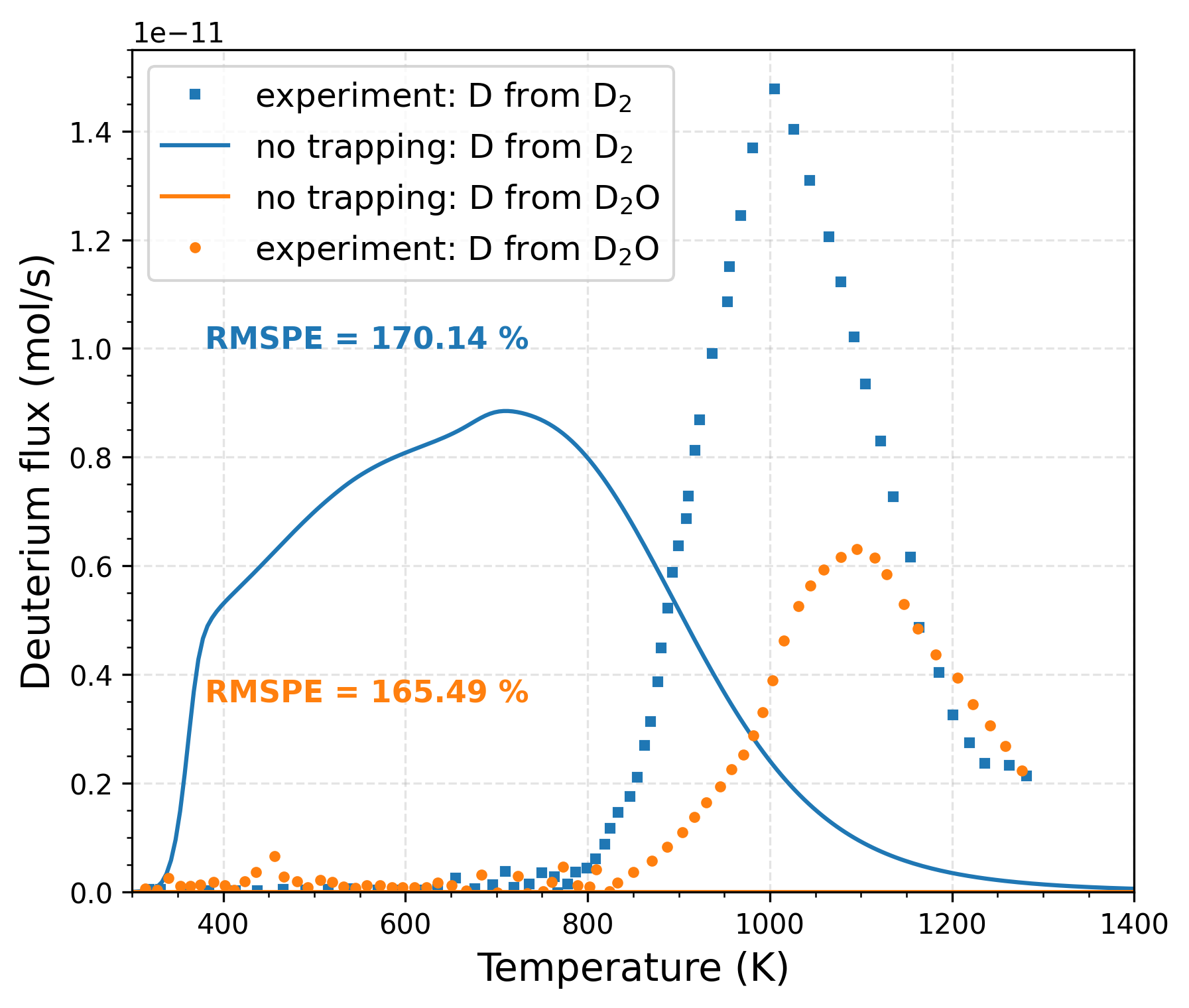
[RMSPE_T2O_dry]
type = ParsedPostprocessor
pp_names = 'timestep_number sum_difference_square_T2O_dry sum_experiment_data_T2O_dry'
expression = 'sqrt(sum_difference_square_T2O_dry / timestep_number) / (sum_experiment_data_T2O_dry / timestep_number + 1e-10)'
execute_on = 'TIMESTEP_END'
[]
[RMSPE_T2_dry]
type = ParsedPostprocessor
pp_names = 'timestep_number sum_difference_square_T2_dry sum_experiment_data_T2_dry'
expression = 'sqrt(sum_difference_square_T2_dry / timestep_number) / (sum_experiment_data_T2_dry / timestep_number + 1e-10)'
execute_on = 'TIMESTEP_END'
[]
#### Postprocessors optimization for wet
[pp_experiment_data_T2O_wet_interpolation]
type = FunctionValuePostprocessor
function = experiment_data_T2O_wet_scale_function
execute_on = 'INITIAL TIMESTEP_END'
[]
[pp_simulation_data_T2O_wet]
type = FunctionValuePostprocessor
function = T_flux_T2O_wet_function
execute_on = 'INITIAL TIMESTEP_END'
[]
[pp_experiment_data_T2_wet_interpolation]
type = FunctionValuePostprocessor
function = experiment_data_T2_wet_scale_function
execute_on = 'INITIAL TIMESTEP_END'
[]
[pp_simulation_data_T2_wet]
type = FunctionValuePostprocessor
function = T_flux_T2_wet_function
execute_on = 'INITIAL TIMESTEP_END'
[]
[differece_square_T2O_wet]
type = FunctionValuePostprocessor
function = difference_square_T2O_wet_function
execute_on = 'INITIAL TIMESTEP_END'
[]
[differece_square_T2_wet]
type = FunctionValuePostprocessor
function = difference_square_T2_wet_function
execute_on = 'INITIAL TIMESTEP_END'
[]
[sum_difference_square_T2O_wet]
type = CumulativeValuePostprocessor
postprocessor = differece_square_T2O_wet
execute_on = 'INITIAL TIMESTEP_END'
[]
[sum_difference_square_T2_wet]
type = CumulativeValuePostprocessor
postprocessor = differece_square_T2_wet
execute_on = 'INITIAL TIMESTEP_END'
[]
[sum_experiment_data_T2O_wet]
type = CumulativeValuePostprocessor
postprocessor = pp_experiment_data_T2O_wet_interpolation
execute_on = 'INITIAL TIMESTEP_END'
[]
[sum_experiment_data_T2_wet]
type = CumulativeValuePostprocessor
postprocessor = pp_experiment_data_T2_wet_interpolation
execute_on = 'INITIAL TIMESTEP_END'
[]
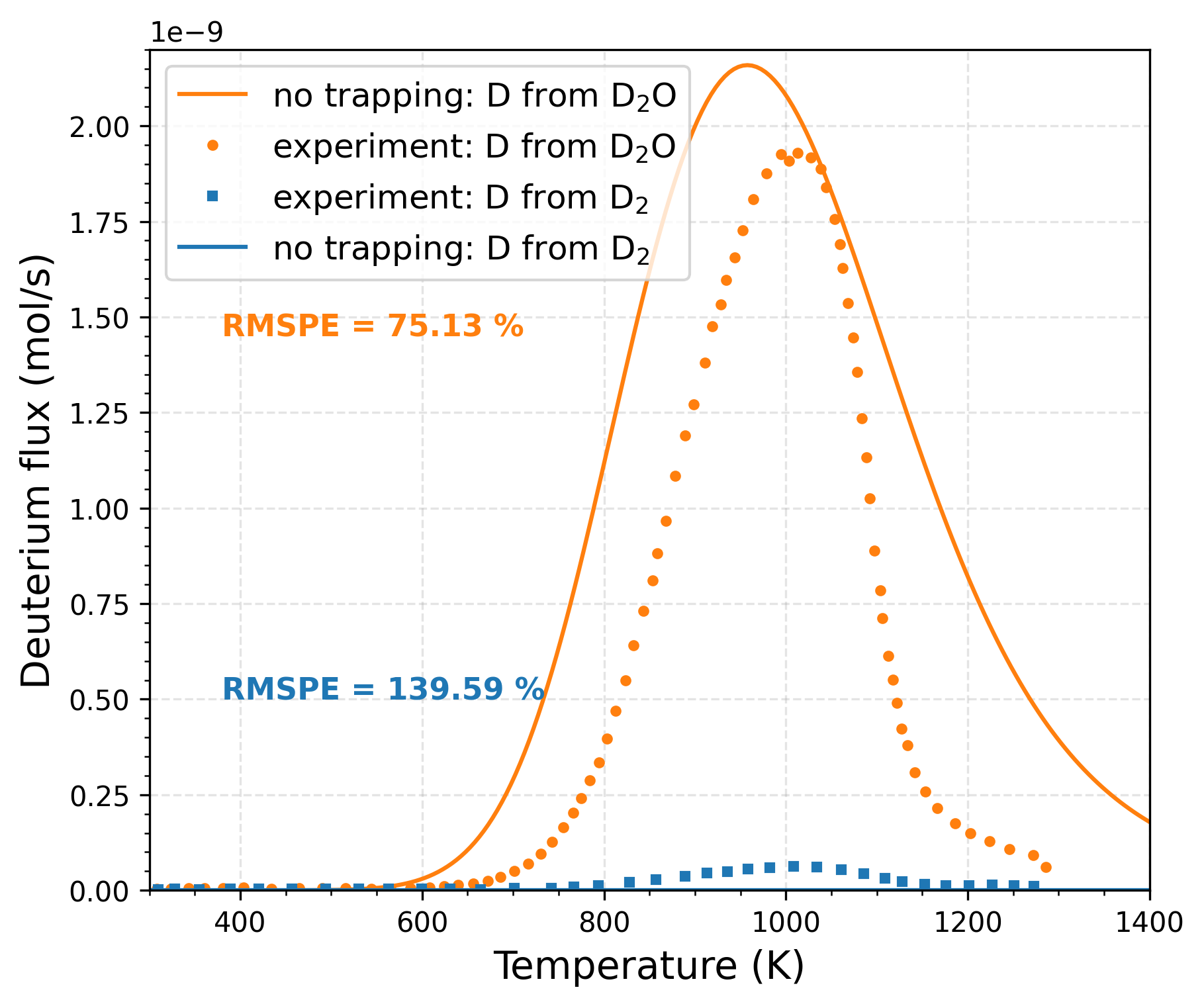
[RMSPE_T2O_wet]
type = ParsedPostprocessor
pp_names = 'timestep_number sum_difference_square_T2O_wet sum_experiment_data_T2O_wet'
expression = 'sqrt(sum_difference_square_T2O_wet / timestep_number) / (sum_experiment_data_T2O_wet / timestep_number + 1e-10)'
execute_on = 'TIMESTEP_END'
[]
[RMSPE_T2_wet]
type = ParsedPostprocessor
pp_names = 'timestep_number sum_difference_square_T2_wet sum_experiment_data_T2_wet'
expression = 'sqrt(sum_difference_square_T2_wet / timestep_number) / (sum_experiment_data_T2_wet / timestep_number + 1e-10)'
execute_on = 'TIMESTEP_END'
[]
[log_inverse_error]
type = ParsedPostprocessor
pp_names = 'RMSPE_T2O_wet RMSPE_T2_wet RMSPE_T2O_dry RMSPE_T2_dry'
expression = 'if(RMSPE_T2O_wet>0,
if(RMSPE_T2_wet>0,
if(RMSPE_T2O_dry>0,
if(RMSPE_T2_dry>0, log(1 / (RMSPE_T2O_wet + RMSPE_T2_wet + RMSPE_T2O_dry + RMSPE_T2_dry)), -20), -20), -20), -20)'
execute_on = 'INITIAL TIMESTEP_END'
[]
[]
[Controls]
[stochastic]
type = SamplerReceiver
[]
[]
[Executioner]
type = Transient
scheme = bdf2
solve_type = NEWTON
petsc_options_iname = '-pc_type -snes_type'
petsc_options_value = 'lu vinewtonrsls'
nl_rel_tol = 1e-7
nl_abs_tol = 1e-10
end_time = ${endtime}
automatic_scaling = true
compute_scaling_once = true
line_search = none
error_on_dtmin = false
nl_max_its = 10
[TimeStepper]
type = IterationAdaptiveDT
dt = ${dt_start_charging}
optimal_iterations = 7
growth_factor = 1.1
cutback_factor = 0.9
cutback_factor_at_failure = 0.9
timestep_limiting_postprocessor = max_time_step_size
[]
[]
[Debug]
show_var_residual_norms = true
[]
[Outputs]
[csv]
type = CSV
[]
[exodus]
type = Exodus
start_time = ${fparse dissolve_duration + cooldown_duration}
[]
[]